Download
1 / 20
200 likes | 378 Views
The SHEq code: an equilibrium calculation tool for SHAx states. Emilio Martines, Barbara Momo Consorzio RFX, Associazione Euratom-ENEA sulla fusione, Padova, Italy. DAx. magnetic axis. O-point. SHAx. X-point. new helical axis. SHAx states.

E N D
The SHEq code: an equilibrium calculation tool for SHAx states Emilio Martines, Barbara Momo Consorzio RFX, Associazione Euratom-ENEA sulla fusione, Padova, Italy
DAx magnetic axis O-point SHAx X-point new helical axis SHAx states Experimentally found in RFX-mod [R. Lorenzini et al., PRL 101, 025005 (2008)] Single Helical Axis Double Axis
The Single Helicity Equilibrium (SHEq) code • The SHEq code was an important ingredient of the Nature Physics paper [R. Lorenzini et al., Nature Phys. 5, 570 (2009)]. • The code computes for SHAx states in toroidal geometry: • Shape of flux surfaces (also for DAx); • Average over flux surfaces of any quantity; • Safety factor profile; • Metric coefficients to be used by ASTRA for transport calculations. • Limitations: • Force-free; • First order in dominant mode amplitude; • Fixed model for parallel current density profile (a-Q0).
The approach Canonical magnetic field representation: toroidal flux poloidal flux In general, F=F(r,,) and = (r, ,). In Single Helicity, F=F(r,u) and = (r,u), where u = m-n. In this case, it can be shown that B·=0, where the helical flux is defined as Thus, the contours of the helical flux give the shape of the flux surfaces. The SHEq code uses the helical flux obtained as superposition of an axysymmetric equilibrium and of the dominant mode (1,7) eigenfunction given by Newcomb’s equation, as in: P. Zanca and D. Terranova, Plasma Phys. Control. Fusion 46, 1115 (2004)
circular cross section Shafranov shift Origin of “geometric” and “flux” coordinates Origin of cylindrical coordinates (torus axis) FLUX GEOM. Vacuum vessel center Step 1: Axysymmetric equilibrium Assuming circular flux surfaces, one defines “geometric” coordinates (r,,) describing the shifted surfaces, and then redefines the poloidal angle, obtaining “flux” coordinates (r,f,), i.e. straight field lines coordinates, through f = + (r, ). Equations are derived to compute F0(r), 0(r) and (r), assuming a (r) profile given by the -0 model.
Step 2: Newcomb’s equation solution Include perturbations: Calculate amplitudes and phases of perturbed fluxes m,n and fm,n solving the first-order force balance equation J1B0 + J0B1= 0. For each n, coupled equations for m = -1, 0, 1, 2 are obtained. The solution involves an unknown derivative discontinuity on resonant surfaces. Thus, it is required to impose both the Br and B harmonics at plasma edge, obtained from measurements. Notice that the perturbed fluxes, F(r,f,) and (r,f,), are not flux functions any more. However, for the Single Helicity case, = m -nF is a flux function.
Example of mapping of Te and SXR over flux surfaces Te SXR emissivity reproduced from: R. Lorenzini et al., Nature Phys. 5, 570 (2009)
label flux surface angular variables Z Helical coordinates: P Z ZA helical axis Poloidal-like angle RA R R Toroidal angle 3D Equilibrium NB: Helical coordinates for flux surface averaging We use c as “radius” and define a new poloidal angle, , with respect to the new axis. Coordinate origin on helical axis Helical flux (flux surface label) Geometric relationship linking helical coordinates to cylindrical coordinates.
Relate the Jacobian to that of the flux coordinates defined by Zanca and Terranova for the axisymmetric equilibrium Result: Positive defined Jacobian >0 Relating helical coordinates to cartesian ones In order to compute flux surface averages, we need to write the metric tensor elements of the new coordinate system, and in particular the Jacobian. Average of a function F(x): Helical coordinate Jacobian Function remapped on the helical coordinates
Examples of flux surface averages We use as “radial” coordinate the square root of the normalized helical flux: (now in progress, change to poloidal flux, for better comparison with VMEC) Btor Jtor Bpol Jpol
V’ g11 element of metric tensor Example: power balance g11 and V’ are computed by SHEq and fed into ASTRA, which calculates the thermal conductivity. courtesy of Rita Lorenzini
Safety factor The safety factor q is computed using the formal equivalence to Hamiltonian dynamics (method suggested by D. F. Escande). (equivalence: H, F p, fq, t) By substitution: (new equivalence: H, F p, u q, t) We have now a “time-independent Hamiltonian” (F,u). Flux coordinates (straight field lines) in Hamiltonian language are action-angle coordinates. Compute action by averaging over constant- orbit: The motion frequency in action-angle coordinates is: Taking into account the n-fold twisting of the helical axis, the actual rotational transform can be computed as:
Example of safety factor in SHAx states The safety factor takes an almost constant value around 1/8 inside the bean-shaped region, where the electron temperature is also flat.
Ohmic constraint In stationary conditions, the parallel Ohm’s law, E·B = j·B, gives where is the electrostatic potential and Vt is the toroidal loop voltage. Flux-surface averaging removes the electrostatic term, so that uniform Zeff profile The SHEq equilibria do not satisfy the Ohmic constraint. the (,0) model is not adequate. (many thanks to A. Boozer for useful discussions)
Outlook The SHEq code is operational for RFX-mod. It also provides input for VMEC calculations (at the moment essential to ensure VMEC convergence). Possible improvements include: • Write output in format which can be read by other codes (DKES, ....). • Adapt profile, so as to reduce the discrepancy in Ohmic constraint. • Better treatment of DAx cases (presently only flux surface plotting). • More ambitiously, iteratively compute an ohmic equilibrium, which simultaneously satisfies force balance and parallel Ohm’s law. The use of SHEq on other RFP devices is encouraged (requires some adaptation, but we are eager to collaborate). A closer interaction with the stellarator community would also be important.
An off-topic slide Results from RFX-mod point to the need of providing the RFP configuration with a divertor. We have recently proposed to use the intrinsic m=0 islands to build, for a RFP operating in SHAx state, the equivalent of the “island divertor” used in stellarators. [E. Martines et al., Nucl. Fusion 50, 035014 (2010)] Limiter-like condition Divertor-like condition This is an issue to be considered when designing new experiments.