Download
1 / 27
280 likes | 421 Views
Automatically Adapting Programs for Mixed-Precision Floating-Point Computation. Mike Lam and Jeff Hollingsworth University of Maryland, College Park Bronis de Supinski and Matt LeGendre Lawrence Livermore National Lab. Background.

E N D
Automatically Adapting Programs for Mixed-Precision Floating-Point Computation Mike Lam and Jeff Hollingsworth University of Maryland, College Park Bronis de Supinski and Matt LeGendre Lawrence Livermore National Lab
Background • Floating point represents real numbers as (± sgnf × 2exp) • Sign bit • Exponent • Significand (“mantissa” or “fraction”) • Finite precision • Single-precision: 24 bits (~7 decimal digits) • Double-precision: 53 bits (~16 decimal digits) • Introduces rounding error 8 4 32 0 16 IEEE Single Exponent (8 bits) Significand (23 bits) 8 4 64 32 0 16 IEEE Double Exponent (11 bits) Significand (52 bits) 2
Motivation • Double precision is ubiquitous • Necessary for some computations • Lack of easy-to-use techniques for reasoning about precision • Single precision is preferable • Faster computation • Tesla K20X: 2.95 TFlops (singles) vs. 1.31 TFlops (doubles) • Intel Xeon Phi: 2.15 GFlops (singles) vs. 1.07 GFlops (doubles) • Standard CPUs: 2x operations w/ SSE vector operations • Reduced memory pressure • Up to 50% footprint reduction • Data movement is a bottleneck for some domains Desire: Balance speed (singles) with accuracy (doubles) 3
Mixed Precision • Use double precision where necessary • Use single precision where possible • Nearly 2x speedups [Baboulin2008] 1: LU ← PA 2: solve Ly = Pb 3: solve Ux0 = y 4: for k = 1, 2, ... do 5: rk ← b – Axk-1 6: solve Ly = Prk 7: solve Uzk = y 8: xk ← xk-1 + zk 9: check for convergence 10: end for Mixed-precision linear solver algorithm Red text indicates steps performed in double-precision (all other steps are single-precision) 4
Our Goal Use automated analysis techniques to prototype mixed-precision variants and provideinsight about a program’s precision level requirements. 5
Framework CRAFT: Configurable Runtime Analysis for Floating-point Tuning • Static binary instrumentation • Parse binary on disk • Replace or augment floating-point instructions with new code • Rewrite modified binary • Dynamic analysis • Run modified program on representative data set • Produce results and recommendations 6
Previous Work • Cancellation detection [WHIST’11] • Reports loss of precision due to subtraction • Provides insight regarding numerical behavior • Range tracking • Reports per-instruction min/max values • Provides insight regarding low dynamic ranges • Mixed-precision variants • Replaces double-precision instructions and operands • Provides insight regarding precision-level sensitivity 7
Implementation • In-place replacement • Narrowed focus: doubles singles • In-place downcast conversion • Flag in the high bits to indicate replacement 8 4 64 32 0 16 Double downcast conversion 8 4 64 32 0 16 Replaced Double 7 F F 4 D E A D Non-signalling NaN 8 4 32 0 16 Single 8
Example gvec[i,j] = gvec[i,j] * lvec[3] + gvar 1 movsd0x601e38(%rax, %rbx, 8) %xmm0 2 mulsd-0x78(%rsp) * %xmm0 %xmm0 3 addsd-0x4f02(%rip) + %xmm0 %xmm0 4 movsd %xmm0 0x601e38(%rax, %rbx, 8) 9
Example gvec[i,j] = gvec[i,j] * lvec[3] + gvar 1 movsd0x601e38(%rax, %rbx, 8) %xmm0 2 mulss-0x78(%rsp) * %xmm0 %xmm0 3 addss-0x4f02(%rip) + %xmm0 %xmm0 4 movsd %xmm0 0x601e38(%rax, %rbx, 8) 10
Example gvec[i,j] = gvec[i,j] * lvec[3] + gvar 1 movsd0x601e38(%rax, %rbx, 8) %xmm0 check/replace -0x78(%rsp) and %xmm0 2 mulss-0x78(%rsp) * %xmm0 %xmm0 check/replace -0x4f02(%rip) and %xmm0 3 addss-0x4f02(%rip) + %xmm0 %xmm0 4 movsd %xmm0 0x601e38(%rax, %rbx, 8) 11
Replacement Code push %rax push %rbx <for each input operand> <copy input into %rax> mov %rbx, 0xffffffff00000000 and %rax, %rbx # extract high word mov %rbx, 0x7ff4dead00000000 test %rax, %rbx # check for flag je next # skip if replaced <copy input into %rax> cvtsd2ss %rax, %rax # down-cast value or %rax, %rbx # set flag <copy %rax back into input> next: <next operand> pop %rbx pop %rax <replaced instruction> # e.g. addsd => addss 12
Dyninst • Binary analysis framework • Parses executable files (InstructionAPI& ParseAPI) • Inserts instrumentation (DyninstAPI) • Supports full binary modification (PatchAPI) • Rewrites binary executable files (SymtabAPI) dyninst.org 13
Block Editing original instruction in block block splits double single conversion initialization check/replace 14
Overhead 15
Binary Editing Double Precision Mixed Precision Original Binary (“mutatee”) CRAFT (“mutator”) Modified Binary Mixed Config Configuration (parser & GUI) 16
Automated Search • Manual mixed-precision replacement • Hard to use without intuition regarding potential replacements • Automatic mixed-precision analysis • Try lots of configurations (empirical auto-tuning) • Test with user-defined verification routine and data set • Exploit program control structure: replace larger structures (modules, functions) first • If coarse-grained replacements fail, try finer-grained subcomponent replacements 18
NAS Results 22
AMGmk Results • Algebraic MultiGrid microkernel • Multigrid method is iterative and highly adaptive • Good candidate for replacement • Automatic search • Complete conversion (100% replacement) • Manually-rewritten version • Speedup: 175 sec to 95 sec (1.8X) • Conventional x86_64 hardware 24
SuperLU Results • Package for LU decomposition and linear solves • Reports final error residual (useful for threshholding) • Both single- and double-precision versions • Verified manual conversion via automatic search • Used error from provided single-precision version as threshold • Final config matched single-precision profile (99.9% replacement) 25
Future Work • Memory-based analysis • Case studies • Search optimization 26
Conclusion Automated binary modification can build prototype mixed-precision program variants. Automated search can provide insight to focus mixed-precision implementation efforts. 27
Thank you! sf.net/p/crafthpc 28