Quick-Sort

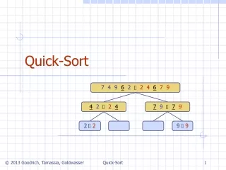
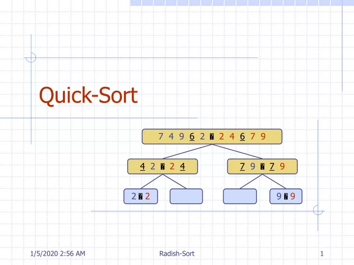
1. 7 4 9 6 2 2 4 6 7 9 4 2 2 4 7 9 7 9 2 2 9 9 Quick-Sort Radish-Sort

2. Outline and Reading • Quick-sort (§10.3) • Algorithm • Partition step • Quick-sort tree • Execution example • Analysis of quick-sort • In-place quick-sort • Summary of sorting algorithms Radish-Sort

3. Quick-sort is a randomized sorting algorithm based on the divide-and-conquer paradigm: Divide: pick a random element x (called pivot) and partition S into L elements less than x E elements equal x G elements greater than x Recur: sort L and G Conquer: join L, Eand G Quick-Sort x x L G E x Radish-Sort

4. Partition Algorithmpartition(S,p) Inputsequence S, position p of pivot Outputsubsequences L,E, G of the elements of S less than, equal to, or greater than the pivot, resp. L,E, G empty sequences x S.remove(p) whileS.isEmpty() y S.remove(S.first()) ify<x L.insertLast(y) else if y=x E.insertLast(y) else{ y > x } G.insertLast(y) return L,E, G • We partition an input sequence as follows: • We remove, in turn, each element y from S and • We insert y into L, Eor G,depending on the result of the comparison with the pivot x • Each insertion and removal is at the beginning or at the end of a sequence, and hence takes O(1) time • Thus, the partition step of quick-sort takes O(n) time Radish-Sort

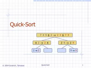
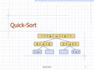
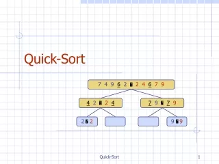
5. Quick-Sort Tree • An execution of quick-sort is depicted by a binary tree • Each node represents a recursive call of quick-sort and stores • Unsorted sequence before the execution and its pivot • Sorted sequence at the end of the execution • The root is the initial call • The leaves are calls on subsequences of size 0 or 1 7 4 9 6 2 2 4 6 7 9 4 2 2 4 7 9 7 9 2 2 9 9 Radish-Sort

6. Execution Example • Pivot selection 7 2 9 4 3 7 6 11 2 3 4 6 7 8 9 7 2 9 4  2 4 7 9 3 8 6 1  1 3 8 6 9 4  4 9 3  3 8  8 2  2 9  9 4  4 Radish-Sort

7. Execution Example (cont.) • Partition, recursive call, pivot selection 7 2 9 4 3 7 6 11 2 3 4 6 7 8 9 2 4 3 1 2 4 7 9 3 8 6 1  1 3 8 6 9 4  4 9 3  3 8  8 2  2 9  9 4  4 Radish-Sort

8. Execution Example (cont.) • Partition, recursive call, base case 7 2 9 4 3 7 6 11 2 3 4 6 7 8 9 2 4 3 1 2 4 7 3 8 6 1  1 3 8 6 11 9 4  4 9 3  3 8  8 9  9 4  4 Radish-Sort

9. Execution Example (cont.) • Recursive call, …, base case, join 7 2 9 4 3 7 6 11 2 3 4 6 7 8 9 2 4 3 1  1 2 3 4 3 8 6 1  1 3 8 6 11 4 334 3  3 8  8 9  9 44 Radish-Sort

10. Execution Example (cont.) • Recursive call, pivot selection 7 2 9 4 3 7 6 11 2 3 4 6 7 8 9 2 4 3 1  1 2 3 4 7 9 7 1  1 3 8 6 11 4 334 8  8 9  9 9  9 44 Radish-Sort

11. Execution Example (cont.) • Partition, …, recursive call, base case 7 2 9 4 3 7 6 11 2 3 4 6 7 8 9 2 4 3 1  1 2 3 4 7 9 7 1  1 3 8 6 11 4 334 8  8 99 9  9 44 Radish-Sort

12. Execution Example (cont.) • Join, join 7 2 9 4 3 7 6 1 1 2 3 4 67 7 9 2 4 3 1  1 2 3 4 7 9 7 1779 11 4 334 8  8 99 9  9 44 Radish-Sort

13. Worst-case Running Time • The worst case for quick-sort occurs when the pivot is the unique minimum or maximum element • One of L and G has size n - 1 and the other has size 0 • The running time is proportional to the sum n+ (n- 1) + … + 2 + 1 • Thus, the worst-case running time of quick-sort is O(n2) … Radish-Sort

14. Consider a recursive call of quick-sort on a sequence of size s Good call: the sizes of L and G are each less than 3s/4 Bad call: one of L and G has size greater than 3s/4 A call is good with probability 1/2 Probabilistic Fact: The expected number of coin tosses required in order to get k heads is 2k Hence, for a node of depth i, we expect that i/2 parent nodes are associated with good calls the size of the input sequence for the current call is at most (3/4)i/2n Thus, we have For a node of depth 2log4/3n, the expected size of the input sequence is one The expected height of the quick-sort tree is O(log n) The overall amount or work done at the nodes of the same depth of the quick-sort tree is O(n) Thus, the expected running time of quick-sort is O(n log n) Expected Running Time Radish-Sort

15. In-Place Quick-Sort • Quick-sort can be implemented to run in-place • In the partition step, we use replace operations to rearrange the elements of the input sequence such that • the elements less than the pivot have rank less than h • the elements equal to the pivot have rank between h and k • the elements greater than the pivot have rank greater than k • The recursive calls consider • elements with rank less than h • elements with rank greater than k AlgorithminPlaceQuickSort(S,l,r) Inputsequence S, ranks l and r Output sequence S with the elements of rank between l and rrearranged in increasing order ifl  r return i a random integer between l and r x S.elemAtRank(i) (h,k) inPlacePartition(x) inPlaceQuickSort(S,l,h - 1) inPlaceQuickSort(S,k + 1,r) Radish-Sort

16. Summary of Sorting Algorithms Radish-Sort

17. Radish-Sort 1, c 3, a 3, b 7, d 7, g 7, e        0 1 2 3 4 5 6 7 8 9 B Radish-Sort

18. Outline and Reading • Bucket-sort (§10.5) • Lexicographic order • Lexicographic-sort • Radish-sort (§10.5) • Radicchio-sort • Radiator-sort Radish-Sort

19. Let be S be a sequence of n (key, element) items with keys in the range [0, N- 1] Bucket-sort uses the keys as indices into an auxiliary array B of sequences (buckets) Phase 1: Empty sequence S by moving each item (k, o) into its bucket B[k] Phase 2: For i = 0, …,N -1, move the items of bucket B[i] to the end of sequence S Analysis: Phase 1 takes O(n) time Phase 2 takes O(n+ N) time Bucket-sort takes O(n+ N) time Bucket-Sort AlgorithmbucketSort(S,N) Inputsequence S of (key, element) items with keys in the range [0, N- 1]Outputsequence S sorted by increasing keys B array of N empty sequences whileS.isEmpty() f S.first() (k, o) S.remove(f) B[k].insertLast((k, o)) for i 0 toN -1 whileB[i].isEmpty() f B[i].first() (k, o) B[i].remove(f) S.insertLast((k, o)) Radish-Sort

20. 7, d 1, c 3, a 7, g 3, b 7, e 1, c 3, a 3, b 7, d 7, g 7, e B 0 1 2 3 4 5 6 7 8 9        1, c 3, a 3, b 7, d 7, g 7, e Example • Key range [0, 9] Phase 1 Phase 2 Radish-Sort

21. Key-type Property The keys are used as indices into an array and cannot be arbitrary objects No external comparator Stable Sort Property The relative order of any two items with the same key is preserved after the execution of the algorithm Extensions Integer keys in the range [a, b] Put item (k, o) into bucketB[k - a] String keys from a set D of possible strings, where D has constant size (e.g., names of the 50 U.S. states) Sort D and compute the rank r(k)of each string k of D in the sorted sequence Put item (k, o) into bucket B[r(k)] Properties and Extensions Radish-Sort

22. Lexicographic Order • A d-tuple is a sequence of d keys (k1, k2, …, kd), where key ki is said to be the i-th dimension of the tuple • Example: • The Cartesian coordinates of a point in space are a 3-tuple • The lexicographic order of two d-tuples is recursively defined as follows (x1, x2, …, xd) < (y1, y2, …, yd)x1 <y1 x1=y1 (x2, …, xd) < (y2, …, yd) I.e., the tuples are compared by the first dimension, then by the second dimension, etc. Radish-Sort

23. Lexicographic-Sort AlgorithmlexicographicSort(S) Inputsequence S of d-tuplesOutputsequence S sorted in lexicographic order for i ddownto 1 stableSort(S, Ci) • Let Ci be the comparator that compares two tuples by their i-th dimension • Let stableSort(S, C) be a stable sorting algorithm that uses comparator C • Lexicographic-sort sorts a sequence of d-tuples in lexicographic order by executing d times algorithm stableSort, one per dimension • Lexicographic-sort runs in O(dT(n)) time, where T(n) is the running time of stableSort Example: (7,4,6) (5,1,5) (2,4,6) (2, 1, 4) (3, 2, 4) (2, 1, 4) (3, 2, 4) (5,1,5) (7,4,6) (2,4,6) (2, 1, 4) (5,1,5) (3, 2, 4) (7,4,6) (2,4,6) (2, 1, 4) (2,4,6) (3, 2, 4) (5,1,5) (7,4,6) Radish-Sort

24. Radish-sort is a specialization of lexicographic-sort that uses bucket-sort as the stable sorting algorithm in each dimension Radish-sort is applicable to tuples where the keys in each dimension i are integers in the range [0, N- 1] Radish-sort runs in time O(d( n+ N)) Radish-Sort AlgorithmradishSort(S, N) Inputsequence S of d-tuples such that (0, …, 0)  (x1, …, xd) and (x1, …, xd)  (N- 1, …, N- 1) for each tuple (x1, …, xd) in SOutputsequence S sorted in lexicographic order for i ddownto 1 bucketSort(S, N) Radish-Sort

25. Radicchio-Sort • Consider a sequence of nb-bit integers x=xb- 1 … x1x0 • We represent each element as a b-tuple of integers in the range [0, 1] and apply radish sort with N= 2 • This algorithm is called radicchio-sort and runs in O(bn) time • With radicchio-sort, we can sort a sequence of Java ints (32-bits) in linear time AlgorithmradicchioSort(S) Inputsequence S of b-bit integers Outputsequence S sorted replace each element x of S with the item (0, x) for i 0 tob - 1 replace the key k of each item (k, x) of S with bit xi of x bucketSort(S, 2) Radish-Sort

26. 1001 1001 1001 0001 0010 0010 0010 1101 0001 1110 1101 1001 0001 0010 1001 1101 0001 0010 1101 1101 1110 1110 1110 1110 0001 Example • Sorting a sequence of 4-bit integers Radish-Sort

27. Radiation-sort The keys are strings of d characters each We represent each key by a d-tuple of integers, where is the ASCII (8-bit integer) or Unicode (16-bit integer) representation of the i-th character and apply radish sort Rant-sort See the textbook Radiator-sort The keys are integers in the range [0, N2- 1] We represent a key as a 2-tuple of digits in the range[0, N- 1] and apply radish-sort Example (N= 10): 75  (7, 5) Example (N= 8): 35  (4, 3) The running time of radiator-sort is O( n+ N) Can be extended to integer keys in the range [0, Nd- 1] Extensions Radish-Sort

28. Conclusion Radish-Sort