Download
1 / 46
480 likes | 786 Views
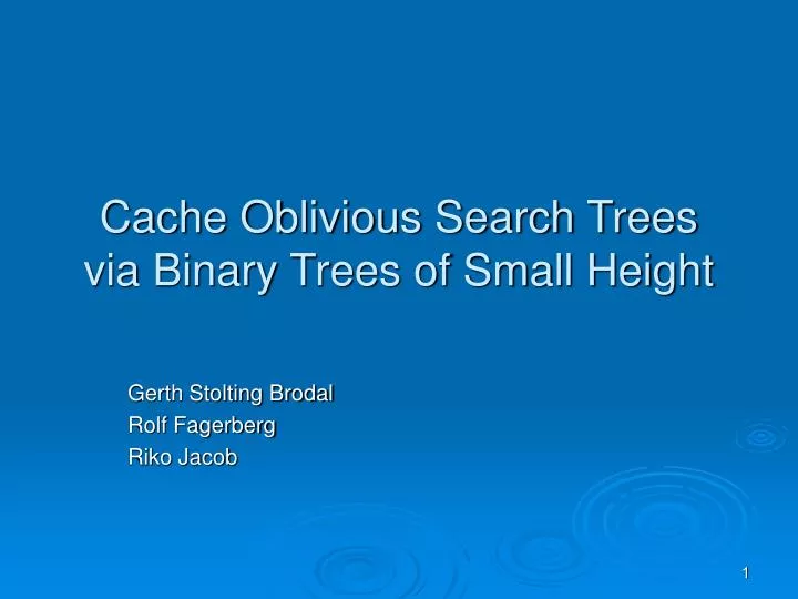
Cache Oblivious Search Trees via Binary Trees of Small Height. Gerth Stolting Brodal Rolf Fagerberg Riko Jacob. Lecture Outline. Motivation General idea & Working methods van Emde Boas memory layout The algorithm Dictionary operations Insertion complexity proof Experiments & Results

E N D
Cache Oblivious Search Trees via Binary Trees of Small Height Gerth Stolting Brodal Rolf Fagerberg Riko Jacob
Lecture Outline • Motivation • General idea & Working methods • van Emde Boas memory layout • The algorithm • Dictionary operations • Insertion complexity proof • Experiments & Results • Summary
Motivation • Modern computers contain a hierarchy of memory levels. • Access time is about 1 [cyc] for registers/ L1 cache, and 100,000 [cyc] for the disk. • The cost of a memory access depends highly on what is the lowest memory level containing the data. • The evolution of CPU speed and memory access time indicates that these differences are likely to increase in the future.
Motivation • Our goal: • To find an implementation for binary search tree that tries to minimize cache misses. • That algorithm will be cache oblivious. • By optimizing an algorithm to one unknown memory level, it is optimized to each memory level automatically !
General idea & Working methods • Definitions: • A tree T1 can be embedded in another tree T2, if T1 can be obtained from T2 by pruning subtrees. • Implicit layout - the navigation between a node and its children is done based on address arithmetic, and not on pointers.
General idea & Working methods • Assume we have a binary search tree. • Embed this tree in a static complete tree. • Save this (complete) tree in the memory in a cache oblivious fashion. • Whenever n is doubled we create a new static tree.
General idea & Working methods • Advantages: • Minimizing memory transfers. • Cache obliviousness • No pointers – better space utilization: • A larger fraction of the structure can reside in lower levels of the memory. • More elements can fit in a cache line. • Disadvantages: • Implicit layout: higher instruction count per navigation – slower.
van Emde Boas memory layout • Recursive definition: • A tree with only one node is a single node record. • If a tree T has two or more nodes: • Divide T to a top tree T0 with height [h(T)/2] and a collection of bottom trees T1,…,Tk with height [h(T)/2] , numbered from left to right. • The van Emde Boas layout of T consist of the v.E.B. layout of T0 followed by the v.E.B. layout of T1,…,Tk
van Emde Boas memory layout • Example :
van Emde Boas memory layout • Example :
van Emde Boas memory layout • Example :
van Emde Boas memory layout • Example : 1
van Emde Boas memory layout • Example : 1 2 3
van Emde Boas memory layout • Example : 1 2 3 4
van Emde Boas memory layout • Example : 1 2 3 4 5 6
van Emde Boas memory layout • Example : 1 2 3 4 7 5 6
van Emde Boas memory layout • Example : 1 2 3 4 7 5 6 8 9
van Emde Boas memory layout • Example : 1 2 3 4 7 10 5 6 8 9 11 12
van Emde Boas memory layout • Example : 1 2 3 4 7 10 13 5 6 8 9 11 12 14 15
The algorithm • Search: • Standard search in a binary tree. • Memory transfers: O(logBn) worst case • Range query: • Standard range query in a binary tree: • Search the smallest element in the range • Make an inorder traversals till you reach an element greater then or equals to the greatest element in the range. • Memory transfers: O(logBn + k/B) worst case
The algorithm • Notations:
The algorithm • Insertions: • Locate the position in T of the new node (regular search) • If d(v) = H+1 we rebalance T Invariant: for the root r:
Rebalancing 1. Find the nearest ancestor w of v with: • That means: find the nearest ancestor of v which is not too dense. • In order to do so we have to calculate • We can do it by a simple traversal – Why?
Rebalancing 2. After having located w we rebalance w as follows: • Create a sorted array of all elements in Tw by an inorder traversal of Tw. • The middle element in the array stored at w. • The smallest (greatest) half elements are recursively redistributed at the left (right) child of w.
Rebalancing • Example : insert 7 8 5 10 4 6
Rebalancing • Example : insert 7 8 5 10 4 6 7
Rebalancing • Example : insert 7 4 5 6 7 8 10 8 5 10 4 6 7
Rebalancing • Example : insert 7 8 10 4 5 6 7 5 10 4 6 7
Rebalancing • Example : insert 7 7 5 8 6 4 4 6 10 7
Rebalancing • Example : insert 7 7 5 8 4 6 10 7
Rebalancing • Example : insert 7 7 5 8 4 6 10 • The next insertion will cause a rebuilding
Insertion complexity • Lemma: A redistribution at v impliesfor all descendants w of v • In other words: after a redistribution at v, for all descendant w • Proof: (induction)
Insertion complexity • Theorem: Insertions require amortized time and amortized memory transfers
Insertion complexity (time) • Proof: • Consider a distribution at a node v, caused by an insertion below v. • for a child w of v :
Insertion complexity (time) • Proof (cont.): • The Lemma argues that immediately after a redistribution at v, for all descendant w of v: • Since the redistribution took place at v:
Insertion complexity (time) • Proof (cont.): • It follows that the number of insertions below w since the last redistribution at v or an ancestor of v is at least: The number of elements at w immediately after the last redistribution at v or at ancestor of v The number of elements in w right now, because w become “dense”
Insertion complexity (time) • Proof (cont.):
Insertion complexity (time) • Proof (cont.): • The redistribution at v takes O(s(v)) which can be covered by elements. Hence, each node is charged at:for each of the mentioned insertions below w.
Insertion complexity (time) • Proof (cont.): • Since each node has at most H ancestors it will be charged at most H times and the amortized complexity will be:
Insertion complexity(memory transfers) • Proof: • A top down search requires O(logBn) memory transfers. • The redistribution itself is like a range query when k=s(v), hence takes:O(max{ 1 , s(v)/B }) memory transfers. • Amortized we got: Finding the ancestor Redistribution at the ancestor
Experiments & Results • The platform: • Two 1[GHz] Pentium 3 processors. • 256[KB] of cache • 1[GB] R.A.M. • Operating system: Linux kernel 2.4.3-12smp. • The experiments – searches with: • Various tree sizes (different n) • Various memory layouts • Implicit and pointer based versions
Experiments & Results • Red: cache aware algs. • Blue: v.E.B layout. • Green: BFS implicit • Black: inorder implicit
Experiments & Results • Red: v.E.B pointer • Green: v.E.B implicit • Black: B.F.S. pointer • Blue: B.F.S. implicit
Summary • We introduced the van Emde Boas layout. • We learned a cache oblivious search tree implementation and its time & memory transfers bounds. • We saw that this implementation is indeed efficient and competitive with cache aware implementations.
Thank you all 14/6/04 Elad Levi