Download
1 / 32
330 likes | 477 Views
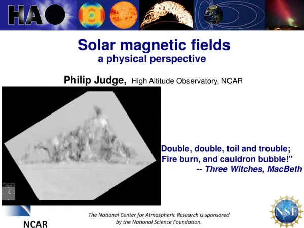
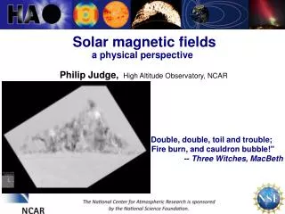
Solar magnetic fields 3. Philip Judge, High Altitude Observatory, NCAR. What is it we really want to know? [Different from stellar case] How do we measure what we want to know? …solar spectropolarimetry. Examples of what we really need/want to know?. Which processes control:

E N D
Solar magnetic fields 3 Philip Judge, High Altitude Observatory, NCAR What is it we really want to know? [Different from stellar case] How do we measure what we want to know? …solar spectropolarimetry
Examples of what we really need/want to know? • Which processes control: • surface field evolution and • the magnetic solar cycle B at the surface, constraints on magnetic flux and helicity∫A.BdV over a solar cycle …requires measurements ofB(r,t) on longer length and time scales
Examples of what we really need/want to know? • what processes control • surface field evolution and • chromospheric/coronal heating • “ dynamics • flaring We should attempt to measure surface B, magnetic free energy (total - potential) Lorentz force j×B, including current sheets requires measurements ofB(r,t) on small length and time scales (flares) up to and including the base of the corona
coronal magnetic free energy can be derived from measurements of magnetic fields at the base in force-free plasma
Conclusion: We must measure vector B • Magnetograph measurements • give BLOS only • yield potential fields (no free energy) in overlying corona • no curl (currents) or uncurl (vector potential) or helicity
An example: Flare physics (Shibata et al 2007) We can measure plasma now Notice- reconnection site It’s time to try to measure the evolving magnetic field
For vector B we must use spectropolarimetry(most lines are not fully split, field is intermittent)
Polarization modulation in time • This is consequential…. unlike in stars, because of • solar evolution (t ~ v / l), l ~ 100 km, v ~ 0.3 cs • atmospheric seeing • let’s look at a rotating waveplate
Spatial as well as temporal modulationremoval of I-> QUV crosstalk with 2 beams In absence of seeing/jitter, a single beam suffices (Solar B SP)
beam splitter D(t) = ΣM3 M2(t) (MC) XT S = M S S = M-1 D ideal solution for Stokes vector Non-Mueller 4xn matrices, n≥4 Diagonality matters In reality we have noise and crosstalk S = (M+Δ)-1 (D+δ), only statistical properties of Δ,δ are knowable
Effects of seeing- bad seeing bad seeing good good+destretched good seeing good seeing, destretched
precise spectropolarimetry is starved of photons! 21
Landi Degl'Innocenti (2012 EWASS meeting): λ = 5000 Å, Δλ = 10 mÅ, T= 5800 K, Δx in arcsec, Δt in seconds, telescope aperture D in meters, T system efficiency: Nphot = 1.2 x 10⁹D2 Δx2 ΔtT Critically sampling R = 1.22 λ/D gives for any aperture D: Nphot = 5 x 10⁶ ΔtT photons/ px Realistically, Δt <10s, T <0.1 so Nphot < 5x 10⁶photons/ px PolarizationsensitivityexceedsNphot-1/2~ 5x 10⁻⁴ Target sensitivity for low (force-free) plasmas: 10-4
Optimalspectropolarimetry • Δx2/R must be 10x larger, e.g. • R=λ/Δλ= 120,000 (24mA @ 500nm, v=c/R = 2.4km/s) • Δx= twice diffraction limit (4x flux) • to give Nphot-1/2~ 5 x 10⁻⁵
… different from stellar case • We must modulate at frequencies >> 1 kHz to remove seeing • e.g. ZIMPOL instrument (charge-caching detector 100 kHz) • otherwise limited to sensitivity P/I > 0.01 %
1st 2nd order in dw/w0=wB/w0
Zeeman line splitting Lites 2000
Zeeman-induced polarization Zeeman parameter ζ: ζ = ωL / ωD, ħωL = μB, ωD= ωline V/c. If ζ << 1: QU ~ ζ2 f” transverseB 180 deg ambiguity V ~ ζf’ longitudinal B
Current density Temperature The “right stuff”: Navarro 2005a,b Inversions of Fe I and Ca II lines in a sunspot, hydrostatic, DST 76cm, SPINOR, sensitivity 1.5x10⁻⁴ “bandwidth limited”
Measuring magnetic fields in solarchromiospheric/coronal (low beta) plasma is hard 200-2000G Uitenbroek 2011 Ca II 854 nm 200-2000G 31
Measuring magnetic fields in solarlow beta plasma is hard Casini, Judge, Schad 2012ApJ Si I/ He I 1083 nm region FIRS/DST, noise ~ 3x10⁻⁴ Instrument fringeremoval using2D PCA