Download

1 / 96
1k likes | 1.34k Views
SIFT. Guest Lecture by Jiwon Kim http://www.cs.washington.edu/homes/jwkim/. SIFT Features and Its Applications. Autostitch Demo. Autostitch. Fully automatic panorama generation Input: set of images Output: panorama(s) Uses SIFT (Scale-Invariant Feature Transform) to find/align images.

E N D
SIFT • Guest Lecture by Jiwon Kim • http://www.cs.washington.edu/homes/jwkim/
Autostitch • Fully automatic panorama generation • Input: set of images • Output: panorama(s) • Uses SIFT (Scale-Invariant Feature Transform) to find/align images
3. Solve for camera parameters • New images initialised with rotation, focal length of best matching image
3. Solve for camera parameters • New images initialised with rotation, focal length of best matching image
4. Blending the panorama • Burt & Adelson 1983 • Blend frequency bands over range l
2-band Blending Low frequency (l > 2 pixels) High frequency (l < 2 pixels)
So, what is SIFT? • Scale-Invariant Feature Transform • David Lowe at UBC • Scale/rotation invariant • Currently best known feature descriptor • Many real-world applications • Object recognition • Panorama stitching • Robot localization • Video indexing • …
SIFT properties • Locality: features are local, so robust to occlusion and clutter • Distinctiveness: individual features can be matched to a large database of objects • Quantity: many features can be generated for even small objects • Efficiency: close to real-time performance
SIFT algorithm overview • Feature detection • Detect points that can be repeatably selected under location/scale change • Feature description • Assign orientation to detected feature points • Construct a descriptor for image patch around each feature point • Feature matching
1. Feature detection • Detect points stable under location/scale change • Build continuous space (x, y, scale) • Approximated by multi-scale Difference-of-Gaussian pyramid • Select maxima/minima in (x, y, scale)
1. Feature detection • Localize extrema by fitting a quadratic • Sub-pixel/sub-scale interpolation using Taylor expansion • Take derivative and set to zero
1. Feature detection • Discard low-contrast/edge points • Low contrast: discard keypoints with < threshold • Edge points: high contrast in one direction, low in the other compute principal curvatures from eigenvalues of 2x2 Hessian matrix, and limit ratio
1. Feature detection • Example • (a) 233x189 image • (b) 832 DOG extrema • (c) 729 left after peak • value threshold • (d) 536 left after testing • ratio of principle • curvatures
2. Feature description • Create histogram of local gradient directions computed at selected scale • Assign canonical orientation at peak of smoothed histogram • Assign orientation to keypoints
2. Feature description • Construct SIFT descriptor • Create array of orientation histograms • 8 orientations x 4x4 histogram array = 128 dimensions
2. Feature description • Advantage over simple correlation • Gradients less sensitive to illumination change • Gradients may shift: robust to deformation, viewpoint change
Performance:stability to noise • Match features after random change in image scale & orientation, with differing levels of image noise • Find nearest neighbor in database of 30,000 features
Performance:stability to affine change • Match features after random change in image scale & orientation, with 2% image noise, and affine distortion • Find nearest neighbor in database of 30,000 features
Performance: distinctiveness • Vary size of database of features, with 30 degree affine change, 2% image noise • Measure % correct for single nearest neighbor match
3. Feature matching • For each feature in A, find nearest neighbor in B A B
3. Feature matching • Nearest neighbor search too slow for large database of 128-dimenional data • Approximate nearest neighbor search: • Best-bin-first [Beis et al. 97]: modification to k-d tree algorithm • Use heap data structure to identify bins in order by their distance from query point • Result: Can give speedup by factor of 1000 while finding nearest neighbor (of interest) 95% of the time
3. Feature matching • Reject false matches • Compare distance of nearest neighbor to second nearest neighbor • Common features aren’t distinctive, therefore bad • Threshold of 0.8 provides excellent separation
3. Feature matching • Now, given feature matches… • Find an object in the scene • Solve for homography (panorama) • …
3. Feature matching • Example: 3D object recognition
3. Feature matching • 3D object recognition • Assume affine transform: clusters of size >=3 • Looking for 3 matches out of 3000 that agree on same object and pose: too many outliers for RANSAC or LMS • Use Hough Transform • Each match votes for a hypothesis for object ID/pose • Voting for multiple bins & large bin size allow for error due to similarity approximation
3. Feature matching • 3D object recognition: solve for pose • Affine transform of [x,y] to [u,v]: • Rewrite to solve for transform parameters:
3. Feature matching • 3D object recognition: verify model • Discard outliers for pose solution in prev step • Perform top-down check for additional features • Evaluate probability that match is correct • Use Bayesian model, with probability that features would arise by chance if object was not present • Takes account of object size in image, textured regions, model feature count in database, accuracy of fit [Lowe01]
Planar recognition • Training images
Planar recognition • Reliably recognized at a rotation of 60° away from the camera • Affine fit approximates perspective projection • Only 3 points are needed for recognition
3D object recognition • Training images
3D object recognition • Only 3 keys are needed for recognition, so extra keys provide robustness • Affine model is no longer as accurate
Applications of SIFT • Object recognition • Panoramic image stitching • Robot localization • Video indexing • … • The Office of the Past • Document tracking and recognition