Common Intersection of Half-Planes in R 2 2

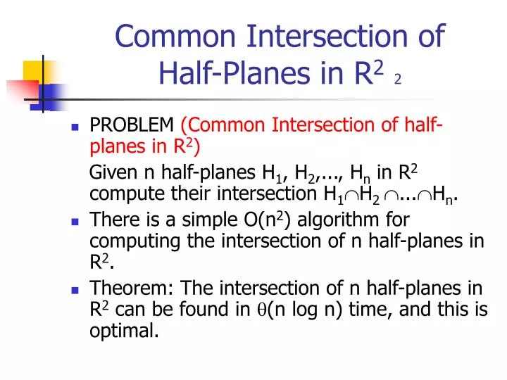
1. Common Intersection of Half-Planes in R22 • PROBLEM (Common Intersection of half-planes in R2) Given n half-planes H1, H2,..., Hn in R2 compute their intersection H1H2 ...Hn. • There is a simple O(n2) algorithm for computing the intersection of n half-planes in R2. • Theorem: The intersection of n half-planes in R2 can be found in (n log n) time, and this is optimal.

2. Common Intersection of Half-Planes in R21 • Theorem: The intersection of n half-planes in R2 can be found in (n log n) time, and this is optimal. • Proof. (1)To show upper bound, we solve it by Divide-and-Conquer T(n) = 2T(n/2) + O(n) = O(n log n) Merge the solutions to sub-problems solutions by finding the intersection of two resulting convex polygons. (2)To prove the lower bound we show that Sorting O(n) Common intersection of half-planes. Given n real numbers x1,..., xn Let Hi: y  2xix – xi2 Once P = H1H2 ...Hn is formed, we may read off the x.'s in sorted Order by reading the slope of successive edges of P.

3. Linear Programming in R2 14 • PROBLEM (2-variable LP) Minimize ax + by, subject to aix + biy + ci 0, i= 1,...,n. • 2-variable LP O(n) Common intersection of half-planes in R2 • Theorem: A linear program in two variables and n constraints can be solved in O(n log n) time.

4. Linear Programming in R2 13 • Theorem: A linear program in two variables and n constraints can be solved in (n). • It can be solved by Prune-and-Search technique. This technique not only discards redundant constraints (i.e. those that are also irrelevant to the half-plane intersection task) but also those constraints that are guaranteed not to contain a vertex extremizing the objective function (referred to as the optimum vertex).

5. Linear Programming in R212 • The 2-variable LP problem Minimize ax + by subject to aix + biy + ci 0, i= 1,...,n. (LP1) can be transformed by setting Y=ax+by & X=x as follows: O(n) Minimize Y subject to iX + iY + ci 0, i= 1,...,n. (LP2) where i=(ai-(a/b)bi) & i= bi/b.

6. Y P X Optimum vertex Linear Programming in R211 • In the new form we have to compute the smallest Y of the vertices of the convex polygon P (feasible region) determined by the constraints.

7. Y P F(X) F+(X) X u1 u2 Linear Programming in R210 • To avoid the construction to the entire boundary of P, we proceed as follows. Depending upon whether i is zero, negative, or positive we partition the index set {1, 2, …, n} into sets I0, I, I+.

8. Linear Programming in R29 • I0: All constraints in I0 are vertical lines and determine the feasible interval for X u1X u2 u1 = max{-ci/i: iI0, i<0} u2 = min{-ci/i: iI0, i>0} • I+: All constraints in I+ define a piecewise upward-convex function F+ = miniI+(i X+i), where i = - (i /i) & i = - (ci /i) • I-: All constraints in I- define a piecewise downward-convex function F- = miniI-(i X+i), where i = - (i /i) & i = - (ci /i)

9. Linear Programming in R28 • Our problem so becomes: O(n) Minimize F-(X) subject to F-(X)  F+(X) (LP3) u1Xu2 • Given X’ of X, the primitive, called evaluation, F+(X’) & F-(X’) can be executed in O(n) • if H(X’) =F-(X’) - F+(X’) > 0, then X’ infeasible • if H(X’) =F-(X’) - F+(X’)  0, then X’ feasible

10. Linear Programming in R27 • Given X’ of X in [u1, u2] , we are able to reach one of the following conclusions in time O(n) • X’ infeasible & no solution to the problem; • X’ infeasible & we know in which side of X’ (right or left) any feasible value of X may lies; • X’ feasible & we know in which side of X’ (right or left) the minimum of F-(X) lies; • X’ achieves the minimum of F-(X);

11. Linear Programming in R26 • We should try to choose abscissa X’ where evaluation takes place s.t. if the algorithm does not immediately terminate, at least a fixed fraction  of currently active constraints can be pruned. We get the overall running time T(n)  i k(1-)i-1n<kn/=O(n)

12. Linear Programming in R25 • We show that the value =1/4 as follows: • At a generic stage assume the stage has M active constraints • let I+& I- be the index set as defined earlier, with | I+|+| I-|=M. • We partition each of I+& I- into pairs of constraints. • For each pair i, j of I+ , O(M) • If i = j (i.e. the corresponding straight lines are parallel) then one can be eliminated. (Fig a) • Otherwise, let Xij denote the abscissa of their intersection • If (Xij < u1 or Xij > u1) then one can be eliminated. (Fig b) • If (u1 Xij  u2) then we retain Xij with no elimination. (Fig c) • For each pair i, j of I- , it is similar to I+ O(M)

13. Eliminated Eliminated Eliminated Y=iX+i Y=jX+j u1 u2 < Xij u2 Xij < u1 Fig c Fig a Fig b Linear Programming in R24

14. Linear Programming in R23 • For all pairs, neither member of which has been eliminated, we compute the abscissa of their abscissa of their intersection. Thus, if k constraints have been eliminated, we have obtained a set S of (M-k)/2 intersection abscissae. O(M) • Find the median X1/2 of S O(M) • If X1/2 is not the extreminzing abscissa, then We test which side of X1/2 the optimum lies. O(M) • So half of the Xij‘s lie in the region which are known not to contain the optimum. For each Xij in the region, one constraint can be eliminated O(M) (Fig d) • This concludes the stage, with the result that at least k+ [(M-k)/2]/2 M/4 constraints have been eliminated.

15. Y P F(X) F+(X) X Xij u1 u2 X1/2 Eliminated Fig d: optimal lies on the left side of X1/2 Linear Programming in R22

16. Linear Programming in R21 • Prune & Search Algorithm for 2-variable LP problem • Transform (LP1) to (LP2) & (LP3) O(M) • For each pair of constraints if (i= i or Xij<u1 or Xij>u2), then eliminate one constraint O(M) • Let S be all the pairs of constraints s.t. u1Xij u2, • Find the median X1/2 of S & test which side of X1/2 the optimum lies O(M) • Half of the Xij‘s lie in the region which are known not to contain the optimum. For each Xij in the region, one constraint can be eliminated. O(M)

17. Common Intersection • Common Intersection of half-planes in R2: (n log n) • 2-varialbe Linear Programming: (n)

18. We must point out that explicit construction of the feasible polytope is not a viable approach to linear programming in higher dimensions because the number of vertices can grow exponentially with dimension. For example, n-dim hypercube has 2n vertices. • The size of Common Intersection of half-spaces in Rk is exponential in k, but the time complexity for k-variable linear programming is polynomial in k. • These two problems are not equivalent in higher dimensions.