Efficiency and Performance Optimization of 3D Lattice Boltzmann Magneto-hydrodynamics

1. 3D Lattice Boltzmann Magneto-hydrodynamics (LBMHD3D) Sam Williams1,2, Jonathan Carter2, Leonid Oliker2, John Shalf2, Katherine Yelick1,2 1University of California Berkeley 2Lawrence Berkeley National Lab samw@cs.berkeley.edu October 26, 2006

2. Outline • Previous Cell Work • Lattice Methods & LBMHD • Implementation • Performance

3. Previous Cell Work

4. Sparse Matrix and Structured Grid PDEs • Double precision implementations • Cell showed significant promise for structured grids, and did very well on sparse matrix codes. • Single precision structured grid on cell was ~30x better than nearest competitor • SpMV performance is matrix dependent (average shown)

5. Quick Introduction to Lattice Methods and LBMHD

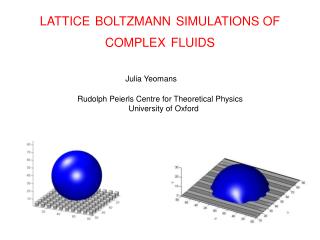
6. Lattice Methods • Lattice Boltzmann models are an alternative to "top-down", e.g. Navier-Stokes and "bottom-up", e.g. molecular dynamics algorithms, approaches • Embedded higher dimensional kinetic phase space • Divide space into a lattice • At each grid point, particles in discrete number of velocity states • Recovery macroscopic quantities from discrete components

7. Lattice Methods (example) • 2D lattice maintains up to 9 doubles (including a rest particle) per grid point instead of just a single scalar. • To update one grid point (all lattice components), one needs a single lattice component from each of its neighbors • Update all grid points within the lattice each time step

8. 4 14 12 2 25 0 9 6 8 18 21 15 22 23 11 10 16 5 13 20 3 1 24 7 19 17 3D Lattice • Rest point (lattice component 26) • 12 edges (components 0-11) • 8 corners (components 12-19) • 6 faces (components 20-25) • Total of 27 components, and 26 neighbors

9. LBMHD3D • Navier-Stokes equations + Maxwell’s equations. • Simulates high temperature plasmas in astrophysics and magnetic fusion • Implemented in Double Precision • Low to moderate Reynolds number

10. LBMHD3D • Originally developed by George Vahala @ College of William and Mary • Vectorized(13x), better MPI(1.2x), and combined propagation&collision(1.1x) by Jonathan Carter @ LBNL • C pthreads, and SPE versions by Sam Williams @ UCB/LBL

11. LBMHD3D (data structures) • Must maintain the following for each grid point: • F : Momentum lattice (27 scalars) • G : Magnetic field lattice (15 cartesian vectors, no edges) • R : macroscopic density (1 scalar) • V : macroscopic velocity (1 cartesian vector) • B : macroscopic magnetic field (1 cartesian vector) • Out of place  even/odd copies of F&G (jacobi) • Data is stored as structure of arrays • e.g. G[jacobi][vector][lattice][z][y][x] • i.e. a given vector of a given lattice component is a 3D array • Good spatial locality, but 151 streams into memory • 1208 bytes per grid point • A ghost zone bounds each 3D grid (to hold neighbor’s data)

12. LBMHD3D (code structure) • Full Application performs perhaps 100K time steps of: • Collision (advance data by one time step) • Stream (exchange ghost zones with neighbors via MPI) • Collision function(focus of this work) loops over 3D grid, and updates each grid point. for(z=1;z<=Zdim;z++){ for(y=1;y<=Ydim;y++){ for(x=1;x<=Xdim;x++){ for(lattice=… // gather lattice components from neighbors for(lattice=… // compute temporaries for(lattice=… // use temporaries to compute next time step }}} • Code performs 1238 flops per point (including one divide) but requires 1208 bytes of data • ~1 byte per flop

13. Implementation on Cell

14. Parallelization • 1D decomposition • Partition outer (ZDim) loop among SPEs • Weak scaling to ensure load balanced • 643 is typical local size for current scalar and vector nodes • requires 331MB • 1K3 (2K3?) is a reasonable problem size (1-10TB) • Need thousands of Cell blades

15. Vectorization • Swap for(lattice=…) and for(x=…) loops • converts scalar operations into vector operations • requires several temp arrays of length XDim to be kept in the local store. • Pencil = all elements in unit stride direction (const Y,Z) • matches well with MFC requirements: gather large number of pencils • very easy to SIMDize • Vectorizing compilers do this and go one step further by fusing the spatial loops and strip mining based on max vector length.

16. Software Controlled Memory • To update a single pencil, each SPE must: • gather 73 pencils from current time (27 momentum pencils, 3x15 magnetic pencils, and one density) • Perform 1238*XDim flops (easily SIMDizable, but not all FMA) • scatter 79 updated pencils (27 momentum pencils, 3x15 magnetic pencils, one density pencil, 3x1 macroscopic velocity, and 3x1 macroscopic magnetic field) • Use DMA List commands • If we pack the incoming 73 contiguously in the local store, a single GETL command can be used • If we pack the outgoing 79 contiguously in the local store, a single PUTL command can be used

17. 5 7 24 3 16 19 24[3] +Plane 16[3] 19[3] +Plane +Pencil 1 13 17 +Plane -Pencil 13[3] 17[3] 8 10 23 20 21 26 9 11 22 -Pencil 23[3] 20[3] 21[3] 26[3] 0 +Pencil 22[3] 0 12 15 4 6 25 2 14 18 12[3] 15[3] -Plane -Pencil -Plane 25[3] -Plane +Pencil 14[3] 18[3] Momentum Lattice YZ Offsets Magnetic Vector Lattice z x y DMA Lists (basically pointer arithmetic) • Create a base DMA get list that includes the inherit offsets to access different lattice elements • i.e. lattice elements 2,14,18 have inherit offset of: -Plane+Pencil • Create even/odd buffer get lists that are just: • base + Y*Pencil + Z*Plane • just ~150 adds per pencil (dwarfed by FP compute time) • Put lists don’t include lattice offsets

18. Double Buffering • Want to overlap computation and communication • Simultaneously: • Load the next pencil • Compute the current pencil • Store the last pencil • Need 307 pencils in the local store at any time • Each SPE has 152 pencils in flight at any time • Full blade has 2432 pencils in flight (up to 1.5MB)

19. Local Computation • Easily SIMDized with intrinsics into vector like operations • DMA offsets are only in the YZ directions, but the lattice method requires an offset in X direction • Used permutes to look forward/back in unit stride direction • worst case to simplify code • No unrolling / software pipelining • Relied on ILP alone to hide latency

20. [0,12] [2,12] [1,12] [0,12] [1,12] [2,12] [2,13] [1,13] [2,13] [0,13] [1,13] [0,13] . . . . . . . . . . . . . . . . . . [1,26] [0,26] [2,26] [1,26] [0,26] [2,26] [0] [0] [1] [1] . . . . . . [26] [26] [2] [2] [1] [1] [0] [0] Putting it all together F[:,:,:,:] G[:,:,:,:,:] Rho[:,:,:] Compute Feq[:,:,:,:] Rho[:,:,:] B[:,:,:,:] Geq[:,:,:,:,:] V[:,:,:,:]

21. Code example for(p=0;p<TotalPencils+3;p++){ // generate list for next/last pencils - - - - - - - - - - - - - - - - - - - - - - - - - - - - - - - - - - - - - - - - - - - if((p>=0)&&(p<TotalPencils )){ DMAGetList_AddToBase(buf^1,(( LoadY*PencilSizeInDoubles)+( LoadZ*PlaneSizeInDoubles))<<3); if( LoadY==Grid.YDim){ LoadY=1; LoadZ++;}else{ LoadY++;} } if((p>=2)&&(p<TotalPencils+2)){ DMAPutList_AddToBase(buf^1,((StoreY*PencilSizeInDoubles)+(StoreZ*PlaneSizeInDoubles))<<3); if(StoreY==Grid.YDim){StoreY=1;StoreZ++;}else{StoreY++;} } // initiate scatter/gather - - - - - - - - - - - - - - - - - - - - - - - - - - - - - - - - - - - - - - - - - - - - - - - - - if((p>=0)&&(p<TotalPencils )) spu_mfcdma32( LoadPencils_F[buf^1][0],(uint32_t)&(DMAGetList[buf^1][0]),(R_0+1)<<3,buf^1,MFC_GETL_CMD); if((p>=2)&&(p<TotalPencils+2)) spu_mfcdma32(StorePencils_F[buf^1][0],(uint32_t)&(DMAPutList[buf^1][0]),(B_2+1)<<3,buf^1,MFC_PUTL_CMD); // wait for previous DMAs - - - - - - - - - - - - - - - - - - - - - - - - - - - - - - - - - - - - - - - - - - - - - - - - - if((p>=1)&&(p<TotalPencils+3)){ mfc_write_tag_mask(1<<(buf)); mfc_read_tag_status_all(); } // compute current (buf) - - - - - - - - - - - - - - - - - - - - - - - - - - - - - - - - - - - - - - - - - - - - - - - - - - if((p>=1)&&(p<TotalPencils+1)){ LBMHD_collision_pencil(buf,ComputeY,ComputeZ); if(ComputeY==Grid.YDim){ComputeY=1;ComputeZ++;}else{ComputeY++;} } buf^=1; }

22. Cell Performance

23. Cell Double Precision Performance • Strong scaling examples • Largest problem, with 16 threads, achieves over 17GFLOP/s • Memory performance penalties if not cache aligned

24. Double Precision Comparison *Collision Only (typically >>85% of time)

25. Conclusions • SPEs attain a high percentage of peak performance • DMA lists allow significant utilization of memory bandwidth (computation limits performance) with little work • Memory performance issues for unaligned problems • Vector style coding works well for this kernel’s style of computation • Abysmal PPE performance

26. Future Work • Implement stream/MPI components • Vary ratio of PPE threads (MPI tasks) to SPE threads • 1 @ 1:16 • 2 @ 1:8 • 4 @ 1:4 • Strip mining (larger XDim) • Better ghost zone exchange approaches • Parallelized pack/unpack? • Process in place • Data structures? • Determine what’s hurting the PPE

27. Acknowledgments • Cell access provided by IBM under VLP • spu/ppu code compiled with XLC & SDK 1.0 • non-cell LBMHD performance provided by Jonathan Carter and Leonid Oliker

28. Questions?