Download
1 / 83
1.01k likes | 1.51k Views
Introduction to Management Science 8th Edition by Bernard W. Taylor III. Chapter 5 Forecasting. Chapter Topics. Forecasting Components Time Series Methods Forecast Accuracy Time Series Forecasting Using Excel Time Series Forecasting Using QM for Windows Regression Methods.

E N D
Introduction to Management Science 8th Edition by Bernard W. Taylor III Chapter 5 Forecasting Chapter 5 - Forecasting
Chapter Topics • Forecasting Components • Time Series Methods • Forecast Accuracy • Time Series Forecasting Using Excel • Time Series Forecasting Using QM for Windows • Regression Methods Chapter 5 - Forecasting
Forecasting Components • A variety of forecasting methods are available for use depending on the time frame of the forecast and the existence of patterns. • Time Frames: • Short-range (one to two months) • Medium-range (two months to one or two years) • Long-range (more than one or two years) • Patterns: • Trend • Random variations • Cycles • Seasonal pattern Chapter 5 - Forecasting
Forecasting Components Patterns (1 of 2) • Trend - A long-term movement of the item being forecast. • Random variations - movements that are not predictable and follow no pattern. • Cycle - A movement, up or down, that repeats itself over a lengthy time span. • Seasonal pattern - Oscillating movement in demand that occurs periodically in the short run and is repetitive. Chapter 5 - Forecasting
trend-line Forecasting Components Patterns (2 of 2) Figure 5.1 Forms of Forecast Movement: (a) Trend, (b) Cycle, (c) Seasonal Pattern, (d) Trend with Seasonal Pattern Chapter 5 - Forecasting
Forecasting Components Forecasting Methods • Times Series - Statistical techniques that use historical data to predict future behavior. • Regression Methods - Regression (or causal ) methods that attempt to develop a mathematical relationship between the item being forecast and factors that cause it to behave the way it does. • Qualitative Methods - Methods using judgment, expertise and opinion to make forecasts. Chapter 5 - Forecasting
Forecasting Components Qualitative Methods • Qualitative methods, the “jury of executive opinion,” is the most common type of forecasting method for long-term strategic planning. • Performed by individuals or groups within an organization, sometimes assisted by consultants and other experts, whose judgments and opinion are considered valid for the forecasting issue. • Usually includes specialty functions such as marketing, engineering, purchasing, etc. in which individuals have experience and knowledge of the forecasted item. • Supporting techniques include the Delphi Method, market research, surveys, etc. Chapter 5 - Forecasting
Time Series Methods Overview • Statistical techniques that make use of historical data collected over a long period of time. • Methods assume that what has occurred in the past will continue to occur in the future. • Forecasts based on only one factor - time. Chapter 5 - Forecasting
Time Series Methods Moving Average (1 of 5) • Moving average uses values from the recent past to develop forecasts. • This dampensor smoothesout random increases and decreases. • Useful for forecasting relatively stable items that do not display any trend or seasonal pattern. • Formula for: Chapter 5 - Forecasting
Time Series Methods Moving Average (2 of 5) • Example: Instant Paper Clip Supply Company forecast of orders for the next month. • Three-month moving average: • Five-month moving average: Chapter 5 - Forecasting
Time Series Methods Moving Average (3 of 5) Figure 5.2 Three- and Five-Month Moving Averages Chapter 5 - Forecasting
Time Series Methods Moving Average (4 of 5) Figure 5.2 Three- and Five-Month Moving Averages Chapter 5 - Forecasting
Time Series Methods Moving Average (5 of 5) • Longer-period moving averages react more slowly to changes in demand than do shorter-period moving averages. • The appropriate number of periods to use often requires trial-and-error experimentation. • Moving average does not react well to changes (trends, seasonal effects, etc.) but is easy to use and inexpensive. • Good for short-term forecasting. Chapter 5 - Forecasting
Time Series Methods Weighted Moving Average (1 of 2) • In a weighted moving average, weights are assigned to the most recent data. • Formula: Chapter 5 - Forecasting
Time Series Methods Weighted Moving Average (2 of 2) • Determining precise weights and number of periods requires trial-and-error experimentation. Chapter 5 - Forecasting
Time Series Methods Exponential Smoothing (1 of 11) • Exponential smoothing weights recent past data more strongly than more distant data. • Two forms: simpleexponential smoothing and adjusted exponential smoothing. • Simple exponential smoothing: Ft + 1 = Dt + (1 - )Ft where: Ft + 1 = the forecast for the next period Dt = actual demand in the present period Ft = the previously determined forecast for the present period = a weighting factor (smoothing constant) use F1 = D1. Chapter 5 - Forecasting
Time Series Methods Exponential Smoothing (2 of 11) • The most commonly used values of are between.10 and .50. • Determination of is usually judgmental and subjective and often based on trial-and -error experimentation. Chapter 5 - Forecasting
Time Series Methods Exponential Smoothing (3 of 11) Example: PM Computer Services (see Table 5.4). • Exponential smoothing forecasts using smoothing constant of .30. • Forecast for period 2 (February): F2 = D1 + (1- )F1 = (.30)(37) + (.70)(37) = 37 units • Forecast for period 3 (March): F3 = D2 + (1- )F2 = (.30)(40) + (.70)(37) = 37.9 units Chapter 5 - Forecasting
Time Series Methods Exponential Smoothing (4 of 11) Using F1 = D1 Table 5.4 Exponential Smoothing Forecasts, = .30 and = .50 Chapter 5 - Forecasting
Time Series Methods Exponential Smoothing (5 of 11) • The forecast that uses the higher smoothing constant (.50) reacts more strongly to changes in demand than does the forecast with the lower constant (.30). • Both forecasts lag behind actual demand. • Both forecasts tend to be consistently lower than actual demand. • Low smoothing constants are appropriate for stable data without trend; higher constants appropriate for data with trends. Chapter 5 - Forecasting
Time Series Methods Exponential Smoothing (6 of 11) Figure 5.3 Exponential Smoothing Forecasts Chapter 5 - Forecasting
Time Series Methods Exponential Smoothing (7 of 11) • Adjusted exponential smoothing: exponential smoothing with a trend adjustment factor added. • Formula: AFt + 1 = Ft + 1 + Tt+1 where: Tt = an exponentially smoothed trend factor: Tt + 1 = (Ft + 1 - Ft) + (1 - )Tt Tt = the last (previous) period’s trend factor = smoothing constant for trend ( a value between zero and one). • Reflects the weight given to the most recent trend data. • Determined subjectively. Chapter 5 - Forecasting
Time Series Methods Exponential Smoothing (8 of 11) Example: PM Computer Services exponential smoothed forecasts with = .50 and = .30 (see Table 5.5). • Start with T2 = 0.00 • Adjusted forecast for period 3: T3 = (F3 - F2) + (1 - )T2 = (.30)(38.5 - 37.0) + (.70)(0) = 0.45 AF3 = F3 + T3 = 38.5 + 0.45 = 38.95 Chapter 5 - Forecasting
Time Series Methods Exponential Smoothing (9 of 11) Tt + 1 = (Ft + 1 - Ft) + (1 - )Tt Table 5.5 Adjusted Exponentially Smoothed Forecast Values Chapter 5 - Forecasting
Time Series Methods Exponential Smoothing (10 of 11) • Adjusted forecast is consistently higher than the simple exponentially smoothed forecast. • It is more reflective of the generally increasing trend of the data. Chapter 5 - Forecasting
Time Series Methods Exponential Smoothing (11 of 11) Figure 5.4 Adjusted Exponentially Smoothed Forecast Chapter 5 - Forecasting
Time Series Methods Linear Trend Line (1 of 5) • When demand displays an obvious trend over time, a least squares regression line , orlinear trend line, can be used to forecast. • Formula: Chapter 5 - Forecasting
Time Series Methods Linear Trend Line (2 of 5) Example: PM Computer Services (see Table 5.6) Chapter 5 - Forecasting
Time Series Methods Linear Trend Line (3 of 5) Table 5.6 Least Squares Calculations Chapter 5 - Forecasting
Time Series Methods Linear Trend Line (4 of 5) • A trend line does not adjust to a change in the trend as does the exponential smoothing method. • This limits its use to shorter time frames in which trend will not change. Chapter 5 - Forecasting
Time Series Methods Linear Trend Line (5 of 5) Figure 5.5 Linear Trend Line Chapter 5 - Forecasting
Time Series Methods Seasonal Adjustments (1 of 4) • A seasonal pattern is a repetitive up-and-down movement in demand. • Seasonal patterns can occur on a monthly, weekly, or daily basis. • A seasonally adjusted forecast can be developed by multiplying the normal forecast by a seasonal factor. • A seasonal factor can be determined by dividing the actual demand for each seasonal period by total annual demand: Si =Di/D Chapter 5 - Forecasting
Time Series Methods Seasonal Adjustments (2 of 4) • Seasonal factors lie between zero and one and represent the portion of total annual demand assigned to each season. • Seasonal factors are multiplied by annual demand to provide adjusted forecasts for each period. Chapter 5 - Forecasting
Time Series Methods Seasonal Adjustments (3 of 4) • Example: Wishbone Farms Table 5.7 Demand for Turkeys at Wishbone Farms S1 = D1/ D = 42.0/148.7 = 0.28 S2 = D2/ D = 29.5/148.7 = 0.20 S3 = D3/ D = 21.9/148.7 = 0.15 S4 = D4/ D = 55.3/148.7 = 0.37 Chapter 5 - Forecasting
Time Series Methods Seasonal Adjustments (4 of 4) • Multiply forecasted demand for entire year by seasonal factors to determine quarterly demand. • Forecast for entire year (trend line for data in Table 5.7): y = 40.97 + 4.30x = 40.97 + 4.30(4) = 58.17 • Seasonally adjusted forecasts: SF1 = (S1)(F5) = (.28)(58.17) = 16.28 SF2 = (S2)(F5) = (.20)(58.17) = 11.63 SF3 = (S3)(F5) = (.15)(58.17) = 8.73 SF4 = (S4)(F5) = (.37)(58.17) = 21.53 Note the potential for confusion: the Si are “seasonal factors” (fractions), whereas the SFi are “seasonally adjusted forecasts” (commodity values)! Chapter 5 - Forecasting
Forecast Accuracy Overview • Forecasts will always deviate from actual values. • Difference between forecasts and actual values referred to as forecast error. • Would like forecast error to be as small as possible. • If error is large, either technique being used is the wrong one, or parameters need adjusting. • Measures of forecast errors: • Mean Absolute deviation (MAD) • Mean absolute percentage deviation (MAPD) • Cumulative error (E-bar) • Average error, or bias (E) Chapter 5 - Forecasting
Forecast Accuracy Mean Absolute Deviation (1 of 7) • MAD is the average absolute difference between the forecast and actual demand. • Most popular and simplest-to-use measures of forecast error. • Formula: Chapter 5 - Forecasting
Forecast Accuracy Mean Absolute Deviation (2 of 7) Example: PM Computer Services (see Table 5.8). • Compare accuracies of different forecasts using MAD: Chapter 5 - Forecasting
Forecast Accuracy Mean Absolute Deviation (3 of 7) Table 5.8 Computational Values for MAD Chapter 5 - Forecasting
Forecast Accuracy Mean Absolute Deviation (4 of 7) • The lower the value of MAD relative to the magnitude of the data, the more accurate the forecast. • When viewed alone, MAD is difficult to assess. • Must be considered in light of magnitude of the data. Chapter 5 - Forecasting
Forecast Accuracy Mean Absolute Deviation (5 of 7) • Can be used to compare accuracy of different forecasting techniques working on the same set of demand data (PM Computer Services): • Exponential smoothing ( = .50): MAD = 4.04 • Adjusted exponential smoothing ( = .50, = .30): MAD = 3.81 • Linear trend line: MAD = 2.29 • Linear trend line has lowest MAD; increasing from .30 to .50 improved smoothed forecast. Chapter 5 - Forecasting
Forecast Accuracy Mean Absolute Deviation (6 of 7) • A variation on MAD is the mean absolute percent deviation(MAPD). • Measures absolute error as a percentage of demand rather than per period. • Eliminates problem of interpreting the measure of accuracy relative to the magnitude of the demand and forecast values. • Formula: Chapter 5 - Forecasting
Forecast Accuracy Mean Absolute Deviation (7 of 7) MAPD for other three forecasts: Exponential smoothing ( = .50): MAPD = 8.5% Adjusted exponential smoothing ( = .50, = .30): MAPD = 8.1% Linear trend: MAPD = 4.9% Chapter 5 - Forecasting
Forecast Accuracy Cumulative Error (1 of 2) • Cumulative error is the sum of the forecast errors (E =et). • A relatively large positive value indicates forecast is biased low, a large negative value indicates forecast is biased high. • If preponderance of errors are positive, forecast is consistently low; and vice versa. • Cumulative error for trend line is always almost zero, and is therefore not a good measure for this method. • Cumulative error for PM Computer Services can be read directly from Table 5.8. • E = et = 49.31 indicating forecasts are frequently below actual demand. Chapter 5 - Forecasting
Forecast Accuracy Cumulative Error (2 of 2) • Cumulative error for other forecasts: Exponential smoothing ( = .50): E = 33.21 Adjusted exponential smoothing ( = .50, =.30): E = 21.14 • Average error (bias) is the per period average of cumulative error. • Average error for exponential smoothing forecast: • A large positive value of average error indicates a forecast is biased low; a large negative error indicates it is biased high. Chapter 5 - Forecasting
Forecast Accuracy Example Forecasts by Different Measures Table 5.9 Comparison of Forecasts for PM Computer Services • Results consistent for all forecasts: • Larger value of alpha is preferable. • Adjusted forecast is more accurate than exponential smoothing forecasts. • Linear trend is more accurate than all the others. Chapter 5 - Forecasting
Time Series Forecasting Using Excel (1 of 4) Exhibit 5.1 Chapter 5 - Forecasting
Time Series Forecasting Using Excel (2 of 4) Exhibit 5.2 Chapter 5 - Forecasting
Time Series Forecasting Using Excel (3 of 4) Exhibit 5.3 Chapter 5 - Forecasting
Time Series Forecasting Using Excel (4 of 4) Exhibit 5.4 Chapter 5 - Forecasting