Download
1 / 56
570 likes | 715 Views
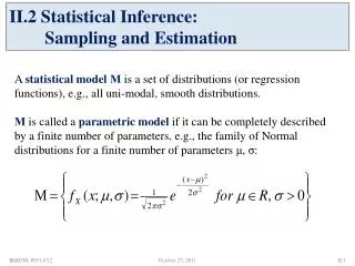
Chapter 5 Statistical Inference Estimation and Testing Hypotheses. 5.1 Data Sets & Matrix Normal Distribution. Data matrix. where n rows X 1 , …, X n are iid. Vec( X ' ) is an np × 1 random vector with. We write More general, we can define matrix normal distribution.

E N D
Chapter 5Statistical Inference Estimation and Testing Hypotheses
5.1 Data Sets & Matrix Normal Distribution Data matrix where n rows X1, …, Xn are iid
Vec(X') is an np×1 random vector with We write More general, we can define matrix normal distribution.
Definition 5.1.1 An n×p random matrix X is said to follow a matrix normal distribution if where In this case, where W=BB', V=AA', Y has i.i.d. elements each following N(0,1).
Theorem 5.5.1 The density function of with W > 0, V >0 is given by where etr(A)= exp(tr(A)). Corollary 1: Let X be a matrix of n observations from Then the density function of X is where
5.2 Maximum Likelihood Estimation A. Review Step 1. The likelihood function
Step 2. Domain (parameter space) The MLE of maximizes over H.
B. Multivariate population Step 1. The likelihood function Step 2. Domain
Step 3. Maximization (a) We can prove that P(B > 0) = 1 if n > p .
(b) We have
(c) Let λ1, …, λp be the eigenvalues of Σ * . The function g(λ)= λ-n/2 e -1/ 2λ arrives its maximum at λ=1/n. The function L(Σ *) arrives its maximum at λ1 =1/n, …, λp =1/n and (d) The MLE of Σ is
Theorem 5.2.1 Let X1, …, Xn be a sample from with n > p and . Then the MLEs of are respectively, and the maximum likelihood is
Theorem 5.2.2 • Under the above notations, we have • are independent; • is a biased estimator of A unbiased estimator of is recommended by called the sample covariance matrix.
Matalb code: mean, cov, corrcoef Theorem 5.2.3 Let be the MLE of and be a measurable function. Then is the MLE of . Corollary 1 The MLE of the correlations is
5.3 Wishart distribution A. Chi-square distribution Let X1, …, Xn are iid N(0,1). Then , the chi-square distribution with n degrees of freedom or Definition 5.1.1 If x ~ Nn(0, In), then Y= x'x is said to have a chi-square distribution with n degrees of freedom, and write .
B. Wishart distribution (obtained by Wishart in 1928) Definition 5.1.1 Let . Then we said that W= x'x is distributed according to a Wishart distribution .
5.4 Discussion on estimation • Unbiaseness • Let be an estimator of . If is called unbiased estimator of . Theorem 5.4.1 Let X1, …, Xn be a sample from Then are unbiased estimators of and , respectively. Matlab code: mean, cov, corrcoef
B. Decision Theory Then the average of loss is give by That is called the risk function.
Definition 5.4.2 An estimator t(X) is called a minimax estimator of if Example 1 Under the loss function the sample mean is a minimax estimator of .
C. Admissible estimation Definition 5.4.3 An estimator t1(x) is said to be at least as good as another t2(x) if And t1 issaid to be better than or strictly dominates t2if the above inequality holds with strict inequality for at least one .
Definition 5.4.4 • An estimator t*is said to be inadmissible if there exists another estimator t** that is better than t*. An estimator t* is admissible if it is not inadmissible. • The admissibility is a weak requirement. • Under the loss , the sample mean is an inadmissible if the population is • James & Stein pointed out is better than The estimator is called James-Stein estimator.
5.5 Inferences about a mean vector (Ch.5 Textbook) Let X1, …, Xn be iid samples from • Case A: is known. • p = 1 • p > 1
Under the hypothesis H0 , Then Theorem 5.5.1 Let X1, …, Xn be a sample from where is known. The null distribution of under is and the rejection area is
Case B: is unknown. • Suggestion: Replace by the Sample Covariance Matrix S in , i.e. • where • There are many theoretic approaches to find a suitable statistic. One of the methods is the Likelihood Ratio Criterion.
The Likelihood Ratio Criterion (LRC) Step 1 The likelihood function Step 2 Domains
Step 3 Maximization We have obtained By a similar way we can find where under
Then, the LRC is Note
Finally Remark: Let t(x) be a statistic for the hypothesis and f(u) is a strictly monotone function. Then is a statistic which is equivalent to t(x). We write
5.6 T2-statistic Definition 5.6.1 Let and be independent with n > p. The distribution of is called T2 distribution. • The distribution T2 is independent of , we shall write • As
And Theorem 5.6.1 Theorem 5.6.2 The distribution of is invariant under all affine transformations of the observations and the hypothesis
Confidence Region • A 100 (1- )% confidence region for the mean of a p-dimensional normal distribution is the ellipsoid determined by all such that
Proof: X1, …, Xn
Example 5.6.1 (Example 5.2 in Textbook) Perspiration from 20 healthy females was analysis.
We evaluate Comparing the observed with the critical value we see that and consequently, we reject H0 at the 10% level of significance.
Mahalanobis Distance Definition 5.6.1 Let x and y be samples of a population G with mean and covariance matrix The quadratic forms are called Mahalanobis distance (M-distance) between x and y, and x and G, respectively.
5.7 Two Samples Problems (Section 6.3, Textbook) We have two samples from the two populations where are unknown. The LRC is where
Under the hypothesis The confidence region of is where
Example 5.7.1(p.338-339) Jolicoeur and Mosimann (1960) studied the relationship of size and shape for painted turtles. The following table contains their measurements on the carapaces of 24 female and 24 male turtles.
5.8 Multivariate Analysis of Variance • Review • There are k normal populations One wants to test equality of the means
The analysis of variance employs decomposition of sum squares where The testing statistics is
B. Multivariate population (pp295-305) is unknown, one wants to test
I. The likelihood ratio criterion Step 1 The likelihood function Step 2 The domains
Step 3 Maximization where are the total sum of squares and products matrix and the error sum of squares and products matrix, respectively.