Download
1 / 64
640 likes | 657 Views
Learn about photometric aspects, gray-level images, filtering techniques, noise models, image smoothing, and non-linear filtering in image processing. Understand radiometric models, brightness values, and mathematical tools used in image analysis.

E N D
Images • - photometric aspects of image formation • gray level images • linear/nonlinear filtering • edge detection • corner detection CS223, Jana Kosecka
Image Brightness values I(x,y) CS223, Jana Kosecka
Image model Mathematical tools Analysis Linear algebra Numerical methods Set theory, morphology Stochastic methods Geometry, AI, logic Analog intensity function Temporal/spatial sampled function Quantization of the gray levels Point sets Random fields List of image features, regions CS223, Jana Kosecka
Basic Photometry Radiometric model of image formation CS223, Jana Kosecka
Basic ingredients Radiance – amount of energy emitted along certain direction Iradiance – amount of energy received along certain direction BRDF – bidirectional reflectance distribution – portion of the energy coming from direction reflected to direction Lambertian surfaces – the appearance depends only on radiance, not on the viewing direction Image intensity for a Lambertian surface CS223, Jana Kosecka
Images • Images contain noise – sources sensor quality, light • fluctuations, quantization effects CS223, Jana Kosecka
Image Noise Models • Additive noise: most commonly used • Multiplicative noise: • Impulsive noise (salt and pepper): • Noise models: gaussian, uniform • Noise Amount: SNR = s/ n CS223, Jana Kosecka
Image filtering • How can we reduce the noise in the image • Image acquisition noise due to light fluctuations and sensor noise can be reduced by acquiring a sequence of images and averaging them • Computation of simple features • First stage of visual processing CS223, Jana Kosecka
Image Processing 1D signal and its sampled version f = { f(1), f(2), f(3), …, f(n)} f = {0, 1, 2, 3, 4, 5, 5, 6, 10 } CS223, Jana Kosecka
Discrete time system f[x] g[x] h • Maps 1 discrete time signal to another • Special class of systems – linear , time-invariant systems Superposition principle Shift (time) invariant – shift in input causes shift in output CS223, Jana Kosecka
g f h g f filter Convolution sum: unit impluse – if x = 0 it’s 1 and zero everywhere else Every discrete time signal can be written as a sum of scaled and shifted impulses The output the linear system is related to the input and the transfer function via convolution Convolution sum: Notation: CS223, Jana Kosecka
Averaging filter Original image Smoothed image CS223, Jana Kosecka
Averaging filter and 0 everywhere else Box filter Ex. cont. Averaging filter center pixel weighted more CS223, Jana Kosecka
11 10 0 0 1 10 X X X X X X 10 1 0 1 9 11 10 X X 10 10 9 0 2 1 f X X 11 10 9 9 11 10 X X 9 10 11 9 99 11 X X 10 9 9 11 10 10 X X X X X X Convolution in 2D g h 1 1 1 1 1 1 1/9 1 1 1 1/9.(10x1 + 11x1 + 10x1 + 9x1 + 10x1 + 11x1 + 10x1 + 9x1 + 10x1) = 1/9.( 90) = 10 CS223, Jana Kosecka
Example: X X X X X X 11 10 0 0 1 10 7 4 1 10 X X 10 1 0 1 9 11 O X X 10 10 9 0 2 1 I X X 11 10 9 9 11 10 X X 9 10 11 9 99 11 F X X X X X X 10 9 9 11 10 10 1 1 1 1 1 1 1/9 1 1 1 1/9.(10x1 + 0x1 + 0x1 + 11x1 + 1x1 + 0x1 + 10x1 + 0x1 + 2x1) = 1/9.( 34) = 3.7778 CS223, Jana Kosecka
F 1 1 1 1 1 1 1 1 1 Example: X X X X X X 11 10 0 0 1 10 7 4 1 10 X X 10 1 0 1 9 11 O X X 10 10 9 0 2 1 I X X 11 10 9 9 11 10 X 20 X 9 10 11 9 99 11 X X X X X X 10 9 9 11 10 10 1/9 1/9.(10x1 + 9x1 + 11x1 + 9x1 + 99x1 + 11x1 + 11x1 + 10x1 + 10x1) = 1/9.( 180) = 20 CS223, Jana Kosecka
How big should the mask be? • The bigger the mask, • more neighbors contribute • bigger noise spread. • more blurring. • more expensive to compute Limitations of averaging • Signal frequencies shared with noise are lost • Impulsive noise is diffused but not removed CS223, Jana Kosecka
Gaussian Filter • Better option for blurring • The coefficients are samples of a 1D Gaussian. • Gives more weight at the central pixel and less weights to the neighbors. • The further away the neighbors, the smaller the weight. • Gaussian filter Samples from the continuous Gaussian • Gaussian filter is the only one that has the same shape • in the space and frequency domains. • There are no secondary lobes – i.e. a truly low-pass filter CS223, Jana Kosecka
How big should the mask be? • The std. dev of the Gaussian determines the amount of smoothing. • The samples should adequately represent a Gaussian • For a 98.76% of the area, we need m = 5 5.(1/) 2 0.796, m 5 5-tap filter g[x] = [0.136, 0.6065, 1.00, 0.606, 0.136] CS223, Jana Kosecka
Image Smoothing • Convolution with a 2D Gaussian filter • Gaussian filter is separable, convolution can be accomplished as two 1-D convolutions CS223, Jana Kosecka
Non-linear Filtering • Replace each pixel with the MEDIAN value of all the pixels in the neighborhood • Non-linear • Does not spread the noise • Can remove spike noise • Expensive to run CS223, Jana Kosecka
11 10 0 0 1 10 X X X X X X 10 1 0 1 9 11 10 X X 10 10 9 0 2 1 I X X 11 10 9 9 11 10 X X 9 10 11 9 99 11 X X 10 9 9 11 10 10 X X X X X X Example: O median sort 10,11,10,9,10,11,10,9,10 9,9,10,10,10,10,10,11,11 CS223, Jana Kosecka
Example: 11 10 0 0 1 X X X X X 10 X 1 1 10 11 1 0 1 10 10 X 9 X O 10 10 9 0 2 1 X X I 11 10 9 9 11 X X 10 9 10 11 9 99 11 X X 10 9 9 11 10 10 X X X X X X median sort 11,10,0,10,11,1,9,10,0 0,0,1,9,10,10,10,11,11 CS223, Jana Kosecka
Example: 11 10 0 0 1 X X X X X 10 X 10 1 0 1 10 X 9 11 X O 10 10 9 0 2 1 X X I 9 11 10 9 9 11 X X 10 9 10 11 9 99 11 X X 10 10 9 9 11 10 10 X X X X X X median sort 10,9,11,9,99,11,11,10,10 9,9,10,10,10,11,11,11,99 CS223, Jana Kosecka
Image Features Local, meaningful, detectable parts of the image. We will look at edges and corners CS223, Jana Kosecka
Gray value column column Edge Edge Image Features – Edges, Corners • Look for detectable, meaningful parts of the image • Edges are detected at places where the image values exhibit sharp variation CS223, Jana Kosecka
Edge detection (1D) F(x) Edge= sharp variation x F ’(x) Large first derivative x CS223, Jana Kosecka
f(x) X-1 X+1 X -1 0 1 Convolve with: Digital Approximation of 1st derivatives CS223, Jana Kosecka
-1 0 Convolve with: -1 0 1 Convolve with: 1 Edge Detection (2D) Vertical Edges: Horizontal Edges: CS223, Jana Kosecka
Noise Filter Edge Detection Noise cleaning and Edge Detection E(x,y) I(x,y) We need to also deal with noise -> Combine Linear Filters CS223, Jana Kosecka
-1 -1 -1 0 0 0 1 1 1 Noise Smoothing & Edge Detection Convolve with: Noise Smoothing Vertical Edge Detection This mask is called the (vertical) Prewitt Edge Detector Outer product of box filter [1 1 1]T and [-1 0 1] CS223, Jana Kosecka
-1 0 1 -1 0 1 -1 0 1 Noise Smoothing & Edge Detection Convolve with: Horizontal Edge Detection Noise Smoothing This mask is called the (horizontal) Prewitt Edge Detector CS223, Jana Kosecka
-1 0 -1 -2 1 -1 0 -2 0 0 0 2 1 2 0 1 -1 1 Sobel Edge Detector Convolve with: Gives more weight to the center pixels and CS223, Jana Kosecka
0 0 0 0 0 0 0 0 0 0 0 0 0 0 0 0 0 0 0 0 0 0 50 50 0 0 0 50 50 50 0 0 0 100 100 0 0 0 0 50 50 50 0 0 0 0 0 150 150 0 0 50 50 50 0 150 0 150 0 0 0 0 0 0 -1 -1 -1 50 100 150 150 50 100 150 150 0 0 0 -1 1 0 1 -1 -1 0 0 0 0 1 1 1 0 1 Example CS223, Jana Kosecka
Image Derivatives We know better alternative to smoothing Smooth using Gaussian filter g(x) is a 1-D Gaussian filter, g(x,y) – 2-D Gaussian filter Taking a derivative – linear operation (take the derivative of the filter) CS223, Jana Kosecka
Gaussian and its derivative CS223, Jana Kosecka
Vertical edges First derivative CS223, Jana Kosecka
Gradient Magnitude Horizontal edges • Image Gradient CS223, Jana Kosecka
Gradient Orientation CS223, Jana Kosecka
Orientation histogram CS223, Jana Kosecka
Corner detection • A point on a line is hard to match. • Intuition: • Right at corner, gradient is ill defined. • Near corner, gradient has two different values. CS223, Jana Kosecka
Formula for Finding Corners We look at matrix: Gradient with respect to x, times gradient with respect to y Sum over a small region, the hypothetical corner Matrix is symmetric CS223, Jana Kosecka
First, consider case where: • This means all gradients in neighborhood are: • (k,0) or (0, c) or (0, 0) (or off-diagonals cancel). • What is region like if: • ? • ? • and ? • and ? CS223, Jana Kosecka
General Case: In general case from linear algebra, it follows that because C is symmetric: With R being a rotation matrix. So every case can be intrepreted like one on last slide. CS223, Jana Kosecka
Corner Detection • Filter image. • Compute magnitude of the gradient everywhere. • We construct C in a window. • Compute eigenvalues l1 and l2. • If they are both big, we have a corner • Or if smalest eigenvalue of C is bigger than - mark pixel as candidate feature point CS223, Jana Kosecka
Point Feature ExtractionHarris Corner Detector • Alternatively feature quality function (Harris Corner Detector) CS223, Jana Kosecka
Harris Corner Detector - Example CS223, Jana Kosecka
Edge Detection gradient magnitude original image • Compute image derivatives • if gradient magnitude > and the value is a local max. along gradient • direction – pixel is an edge candidate • how to detect one pixel thin edges ? CS223, Jana Kosecka
Th Canny Edge Detector • The magnitude image Es has the magnitudes of the smoothed gradient. • Sigma determines the amount of smoothing. • Es has large values at edges: • Find local maxima CS223, Jana Kosecka
x x Nonmaximum supression • The inputs are Es& Eo Magnitude and orientation • Consider 4 directions D={ 0,45,90,135} wrt x • For each pixel (i,j) do: • Find the direction dD s.t. d Eo(i,j) (normal to the edge) • If {Es(i,j) is smaller than at least one of its neigh. along d} • IN(i,j)=0 • Otherwise, IN(i,j)= Es(i,j) • The output is the thinned edge image IN CS223, Jana Kosecka