Download
1 / 74
740 likes | 753 Views
Understand edge detection, a process crucial for image analysis, to identify object boundaries, reflectance changes, and shadows using difference operators for 2D images. Discover the Canny edge detector and its implementation to track contours and eliminate weak segments.

E N D
Edge detection • Edge detection is the process of finding meaningful transitions in an image. • The points where sharp changes in the brightness occur typically form the border between different objects or scene parts. • Further processing of edges into lines, curves and circular arcs result in useful features for matching and recognition. • Initial stages of mammalian vision systems also involve detection of edges and local features. 2019
Edge detection • Sharp changes in the image brightness occur at: • Object boundaries • A light object may lie on a dark background or a dark object may lie on a light background. • Reflectance changes • May have quite differentcharacteristics – zebrashave stripes, and leopardshave spots. • Cast shadows • Sharp changes in surfaceorientation 2019
Edge models 2019
Difference operators for 2D Adapted from Gonzales and Woods 2019
Difference operators under noise Solution is to smooth first: Adapted from Steve Seitz 2019
Difference operators under noise Differentiation property of convolution: Adapted from Steve Seitz 2019
Difference operators under noise Consider: Laplacian of Gaussian operator Adapted from Steve Seitz 2019
Laplacian of Gaussian Edge detection filters for 2D Gaussian derivative of Gaussian Adapted from Steve Seitz, U of Washington 2019
Difference operators for 2D sigma=4 Laplacian of Gaussianzero crossings Threshold=4 Threshold=1 sigma=2 Adapted from David Forsyth, UC Berkeley 2019
Edge detection • Three fundamental steps in edge detection: • Image smoothing: to reduce the effects of noise. • Detection of edge points: to find all image points that are potential candidates to become edge points. • Edge localization: to select from the candidate edge points only the points that are true members of an edge. 2019
Canny edge detector • Smooth the image with a Gaussian filter with spread σ. • Compute gradient magnitude and direction at each pixel of the smoothed image. • Zero out any pixel response less than or equal to the two neighboring pixels on either side of it, along the direction of the gradient (non-maxima suppression). • Track high-magnitude contours using thresholding (hysteresis thresholding). • Keep only pixels along these contours, so weak little segments go away. 2019
Canny edge detector Original image (Lena) Adapted from Steve Seitz, U of Washington 2019
Canny edge detector Magnitude of the gradient Adapted from Steve Seitz, U of Washington 2019
Canny edge detector Thresholding Adapted from Steve Seitz, U of Washington 2019
Canny edge detector How to turn these thick regions of the gradient into curves? Adapted from Steve Seitz, U of Washington 2019
Non-maxima suppression: Check if pixel is local maximum along gradient direction. Select single max across width of the edge. Requires checking interpolated pixels p and r. This operation can be used with any edge operator when thin boundaries are wanted. Canny edge detector 2019
Canny edge detector Problem: pixels along this edge did not survive the thresholding Adapted from Steve Seitz, U of Washington 2019
Canny edge detector • Hysteresis thresholding: • Use a high threshold to start edge curves, and a low threshold to continue them. 2019
Canny edge detector Adapted from Martial Hebert, CMU 2019
Canny edge detector 2019
Canny edge detector 2019
Canny edge detector • The Canny operator gives single-pixel-wide images with good continuation between adjacent pixels. • It is the most widely used edge operator today; no one has done better since it came out in the late 80s. Many implementations are available. • It is very sensitive to its parameters, which need to be adjusted for different application domains. 2019
Edge linking • Hough transform • Finding line segments • Finding circles • Model fitting • Fitting line segments • Fitting ellipses • Edge tracking 2019
Fitting: main idea • Choose a parametric model to represent a set of features • Membership criterion is not local • Cannot tell whether a point belongs to a given model just by looking at that point • Three main questions: • What model represents this set of features best? • Which of several model instances gets which feature? • How many model instances are there? • Computational complexity is important • It is infeasible to examine every possible set of parameters and every possible combination of features Adapted from Kristen Grauman 2019
Example: line fitting • Why fit lines? • Many objects characterized by presence of straight lines Adapted from Kristen Grauman 2019
Difficulty of line fitting • Extra edge points (clutter), multiple models: • which points go with which line, if any? • Only some parts of each line detected, and some parts are missing: • how to find a line that bridges missing evidence? • Noise in measured edge points, orientations: • how to detect true underlying parameters? Adapted from Kristen Grauman 2019
Voting • It is not feasible to check all combinations of features by fitting a model to each possible subset. • Voting is a general technique where we let each feature vote for all models that are compatible with it. • Cycle through features, cast votes for model parameters. • Look for model parameters that receive a lot of votes. • Noise and clutter features will cast votes too, but typically their votes should be inconsistent with the majority of “good” features. Adapted from Kristen Grauman 2019
Hough transform • The Hough transform is a method for detecting lines or curves specified by a parametric function. • If the parameters are p1, p2, … pn, then the Hough procedure uses an n-dimensional accumulator array in which it accumulates votes for the correct parameters of the lines or curves found on the image. b accumulator image m y = mx + b Adapted from Linda Shapiro, U of Washington 2019
Hough transform: line segments y b b0 m0 x m Image space Hough (parameter) space • Connection between image (x,y) and Hough (m,b) spaces • A line in the image corresponds to a point in Hough space • To go from image space to Hough space: • given a set of points (x,y), find all (m,b) such that y = mx + b Adapted from Steve Seitz, U of Washington 2019
Hough transform: line segments y b y0 x0 x m Image space Hough (parameter) space • Connection between image (x,y) and Hough (m,b) spaces • A line in the image corresponds to a point in Hough space • To go from image space to Hough space: • given a set of points (x,y), find all (m,b) such that y = mx + b • What does a point (x0, y0) in the image space map to? • Answer: the solutions of b = -x0m + y0 • This is a line in Hough space Adapted from Steve Seitz, U of Washington 2019
Hough transform: line segments y b (x1, y1) y0 (x0, y0) b = –x1m + y1 x0 x m Image space Hough (parameter) space What are the line parameters for the line that contains both (x0, y0) and (x1, y1)? • It is the intersection of the lines b = –x0m + y0 and b = –x1m + y1 Adapted from Steve Seitz, U of Washington 2019
c d r Hough transform: line segments • y = mx + b is not suitable (why?) • The equation generally used is: d = r sin(θ) + c cos(θ). d is the distance from the line to origin. θ is the angle the perpendicular makes with the column axis. Adapted from Linda Shapiro, U of Washington 2019
Hough transform: line segments Adapted from Shapiro and Stockman 2019
Hough transform: line segments Adapted from Kristen Grauman 2019
Hough transform: circles • Main idea: The gradient vector at an edge pixel points the center of the circle. • Circle equations: • r = r0 + d sin(θ) r0, c0, d are parameters • c = c0 + d cos(θ) d *(r,c) Adapted from Linda Shapiro, U of Washington 2019
Hough transform: circles Adapted from Shapiro and Stockman 2019
Hough transform: circles https://www.mathworks.com/help/images/ref/imfindcircles.html http://shreshai.blogspot.com.tr/2015/01/matlab-tutorial-finding-center-pivot.html http://docs.opencv.org/2.4/doc/tutorials/imgproc/imgtrans/hough_circle/hough_circle.html 2019
Hough transform: circles Zhao et al., “Oil Tanks Extraction from High Resolution Imagery Using a Directional and Weighted Hough Voting Method”, Journal of the Indian Society of Remote Sensing, September 2015 2019
Model fitting • Mathematical models that fit data not only reveal important structure in the data, but also can provide efficient representations for further analysis. • Mathematical models exist for lines, circles, cylinders, and many other shapes. • We can use the method of least squares for determining the parameters of the best mathematical model fitting the observed data. 2019
Model fitting: line segments Adapted from Martial Hebert, CMU 2019