Download
1 / 32
320 likes | 609 Views
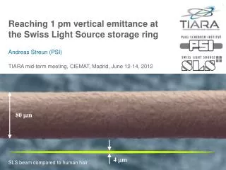
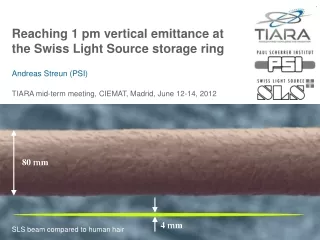
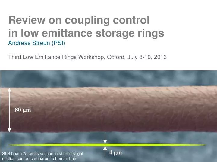
Review on coupling control in low emittance storage rings Andreas Streun (PSI) Third Low Emittance Rings Workshop, Oxford, July 8-10, 2013. 80 m m. 4 m m. SLS beam 2 s cross section in short straight section center compared to human hair. Contents. Coupling and vertical emittance

E N D
Review on coupling control in low emittance storage ringsAndreas Streun (PSI)Third Low Emittance Rings Workshop, Oxford, July 8-10, 2013 80 mm 4 mm SLS beam 2scross section in short straight section center compared to human hair
Contents • Coupling and vertical emittance Quantum emittance Vertical emittance from coupling Properties Measurements Motivations for coupling control Emittances achieved and planned • Methods for coupling control BPM roll error measurements Magnet / girder realignment Model based methods response matrices resonance drive terms LOCO orbit manipulations turn by turn data Model independent methods Coupling control in operation • Summary
Coupling and vertical emittance Quantum emittance = vertical emittance for ideal, flat lattice • direct photon recoil,1/g radiation cone • T. O. Raubenheimer, Tolerances to limit the vertical emittance in future storage rings, SLAC-PUB-4937, Aug.1991 • independent of energy • examples: ASLS 0.35 pmPETRA-III 0.04 pm ultimate limit of vertical emittance quantum emittance << [ < ] coupling G(s) =curvature, Cq = 0.384 pm isomagnetic lattice
Vertical emittance from coupling vertical orbit correctors vertical orbit in quads roll errors of bending magnets • dispersive skew quads • vertical orbit in dispersive sextupoles • roll errors of dispersive quads • A. W. Chao, Evaluation of beam distribution parameters in an electron storage ring, J. Appl. Phys. 50, 595 (1979) • A. Franchi et al., Vertical emittance reduction and preservation in electron storage rings via resonance drive terms correction, PRSTAB 14, 034002 (2011) + LER-2011 Horizontal dipole fields Rotation (torsion) of beam(betatron coupling) Rotation of dispersion Projected e (s) Eigen-e(invariant) Vertical dispersion Apparent e (s) Orbit / BPMs Beam profile monitor
Vertical emittance properties Eigen-e= 9 pm • Apparent-e oscillates around the lattice. • Oscillation amplitude is low for low coupling. • Projected-e changes at skew quad kicks. • Eigen-e is invariant. • Minimization of apparent e at one location (monitor) minimizes eigen-e too: ESRF at large coupling A. Franchi, Coupling correction through beam position data, LER-2011. Eigen-e results, when optimizing on beam size at monitor () vs. optimizing on eigen-e itself ( ). (TRACY simulation, 100 seeds, SLS with 22 skew quads)M. Böge, LER-2010
Vertical emittance measurements Vertical beam size monitor • gives local apparent emittance = [sy(s)]2/by(s) • requires beta function measurement • [dispersion & energy spread measurement too] • different methods... ( A. Saa Hernandez talk) • model based evaluation of measurement • e.g. diffraction effects in imaging 6 mm rms vertical Pinhole camera images before/after coupling correction at DIAMOND C. Thomas, R. Bartolini et al. PRSTAB 13, 022805, (2010) 1-D X-ray diode array camera at CESR-TA J. Shanks, LER-2011
Closest tune approach • Tunes observed on difference resonanceQx- Qy= q : • Betatron coupling from difference resonance • Working point off resonance (but close) • Qx/yuncoupled, Q1/2observed tunes • Vertical emittance(Guignard formula) • Caution • assumes betatron coupling >> vertical dispersion • assumes difference >> sum coupling resonance • single resonance approximation |Q1-Q2| and synear resonance at SPRING-8. M. Takao et al, IPAC-2012, p.1191
Touschek lifetime analysis • Touschek half-life time: T ~ sy • gives sy weighted with local loss rates • in tilted coordinate system measurement of eigen-emittance [?] • Requires dominant Touschek effect • Reduce acceptance by dispersivehorizontal scraper or low RF voltage • Caution • sum coupling resonance may increase vertical emittance and decrease lifetime = linear physical acceptance Beam size vs. lifetime at ALS C. Steier, ICFA-BD-NL #44, p.97
Motivations for coupling control ALS lifetime vs. vertical scraperlow coupling, large dispersionlarge coupling, low dispersionlow coupling, low dispersion, lower ey C. Steier et al., PAC-2003, p.3213 } same ey • measure for quality of optics correction: model vs. machine • damping rings & colliders: maximum bunch density • synchrotron radiation users: • not interested in ey< diffraction (~10 pm for ~10 keV) • suppress betatron coupling: avoid vertical oscillations of Touschek particles allow smaller ID gaps smaller ID periods higher photon energy • increase vertical dispersion: • meet diffraction limit • increase lifetime • feed-back or feed-forwardfor constant beam size
Synchrotron radiation: diffraction limit • Photon emittance = convolution of electron beam and diffraction phase spaces • Diffraction for undulator length L: ed 0.12 l, bd 0.35 L R. Coisson, J. Opt. Eng. 27.3 (1988) W. Joho, SLS note 4/1995 • Electron beamassumption: a = D’ = 0, D = 0[otherwise use effective phase space, convoluted with dispersion] • Optimum matching: • Example: l = 1Å, L = 2 med 12 pm, bd 0.7 m
Emittances achieved and planned 1 km 3 / 6 GeV
Methods for coupling control Overview • Measurement or estimation of BPM roll errorsto avoid “fake” vertical dispersion measurement. • Realignment of girders / magnetsto remove sources of coupling and vertical dispersion. • Model based corrections: • Establish lattice model: multi-parameter fit to orbit response matrix (using LOCO or related methods) to obtain a calibrated model. • Use calibrated model to perform correction or to minimize derived lattice parameters (e.g. vertical emittance) in simulation and apply to machine. • Application to coupling control: correction of vertical dispersion, coupled response matrix, resonance drive terms using skew quads and orbit bumps, or direct minimization of vertical emittance in model. • Model independent corrections: • empirical optimization of observable quantities related to coupling(e.g. beam size, beam life time). • Coupling control in operation: on-line iteration of correction
BPM roll error measurements • BPM roll “fake” vertical dispersion(roll error horiz. disp. > vert. disp.) • Origin: mainly electronics. • Methods: • Local bumps with fast orbit feedback: roll measurement from corrector currents, relative to corrector system. • [LOCO] fit to orbit response matrix:roll estimate in absolute coordinates. “3rd BBA* constant”: BPM sway, heave & roll (*BBA = “beam based alignment”) • Example: Vertical dispersion (ASLS) uncorrected/corrected before () and after () BPM roll subtraction • R. Dowd et al., Achievement of ultra-low vertical emittance in the Australian synchrotron storage ring, PRSTAB-14,012804 (2011)
Magnet / girder realignment • Magnet misalignment = source of coupling • steps between girders: vertical dispersion from vertical corrector dipoles • BBGA (= beam based girder alignment) • Misalignments from orbit response • BAGA (= beam assisted girder alignment) • girder misalignment data from survey. • girder move with stored beam and running orbit feedback. vertical corrector currents confirm move. BAGA (SLS): Corrector strengths (sector 1) before and after girder alignment, and after beam based BPM calibration (BBA) ( girder move deforms vacuum chamber ) • V-Corrector rms strengths reduced by factor 4 (14738 mrad). M. Böge et al., IPAC-2011, p.3035
Model based corrections Response matrix based corrections in general Model • Orbit response matrix from modelM = {x;yBPM/ kCH;CV}. • NBBPMs (x, y) and NH, NV H,V-Correctors: 2NB (NH+ NV) matrix. • Model: sensitivity of the orbit response matrix M on vector of NAparameters A = {ak} local derivatives, resp. Jacobian tensor {M/ ak}. • Rearrange tensor as [2NB (NH+ NV)] NA sensitivity matrix S M = S·A. Measurement • Orbit response matrix M. Correction • Linear: fit vector A of parameters usingSVD-”inversion”: A = S-1·M. • General: vary {ak} to minimize difference (M-M), i.e. S (mij-mij)2/si2.. • Weighting with individual BPM errors si . • Fit result “calibrated model” • Apply inverse of fit result to machine: -{Dak}. • Iterate: measurement correction convergence for M M • Also iterate model for large errors.
Application:Vertical dispersion measurement & correction orbit bump in quadrupole vertical dipole orbit bump in dispersive sextupole dispersive skew quadrupole • Orbit at NBBPMs as function of momentum Dp/p • requires high BPM resolution and low drift (quick measurement) due to limited range of RF change • resolution ~ 0.1 mm, suppression ~ 1 mm (RMS) • Correction with NDdispersive skew quads: NBNDsystem
Application: Beta function correction by quad variation • Example for a not-orbit-based method • direct & independent measurement of beta functions:<bx,y> at NQquadrupoles from tune response. 2NQNQbeta function response matrix from model. • calculation of quad gradient corrections.
Resonance drive terms • Single resonance approximation for large machines • high periodicity, few systematic resonances • working point nearer to difference than to sum coupling resonancee.g. ESRF 36.45/13.39 ESRF method ( A. Franchi, LER-2011), (similar methods at SPRING-8, CESR-TA) • Lattice model from ORM or TBT data • assume many error sources for fitting (quad rolls etc.) • calculate difference and sum coupling resonance drive terms (RDT) and vertical dispersion. • Response matrix for existing skew quad correctors • Empirical weights a1, a2for RDTs vs. vertical dispersion Vertical emittance 2.6 1.1 pm • Definition: mean and rms of 12 beam size monitors
LOCO (linear optics from closed orbit) J. Safranek, Experimental determination of storage ring optics using orbit response measurements, NIM A 368 (1997) 27-36 ICFA beam dynamics news letter #44 (2007) • applied to general optics correction and to coupling control • low statistical error: response matrix = many, highly correlated data • low measurement error: high precision of BPMs in stored beam mode Fit parameters (almost any possible) • quadrupole gradients and roll errors • BPM and corrector calibrations and roll errors • sextupole misalignments • not possible: dipole errors quad misalignments Vertical emittance minimization ( J. Safranek) • minimizing coupled response matrix using existing skew quad correctors does not necessarily give the lowest vertical emittance. • establish model with many skew quad error sources . • use existing skew quads to minimize vertical emittance in model.
Some results of coupling suppression • Example: SSRF[preliminary] (courtesy M. Zhang) • more LOCO calibrated model vertical emittances: • ASLS 0.3 pm (meas. 0.8 0.1 pm) (R. Dowd) • ALS 1.3 pm (meas. ~2 pm) (C. Steier)
Precautions • Choose appropriate orbit excitation • too low: BPM noise –too high: nonlinear response • Choose appropriate filtering (SVD cut-off)and number of model parameters • too high / too few : bad fit – too low / too many : fit to noise • Careful with extrapolations from calibrated model • model: fit all error sources (e.g. quad rolls etc) to ORM • calculation of quantities not directly observed (i.e. lattice functions, e.g. beta functions, vertical emittance) • minimization of these quantities using existingcorrectors (e.g. quad gradients, skew quads) • upload to machine iterate (measure ORM again etc.) • model machine residual error > statistical error • Results will fluctuate with iterations due to model deficiencies. • use average, not value from best iteration... • [better: have independent, direct measurement...] M. Aiba et al., Comparison of linear optics measurements and correction methods at the Swiss Light Source, PRSTAB 16,01202 (2013)
Orbit manipulation: the LET algorithm (“low emittance tuning) • Principle: double linear system • Measurement vectors • vertical orbit horizontal orbit • vertical dispersion horizontal dispersion • off-diagonal (coupling)... diagonal (regular)... ...parts of the orbit response matrix • Knob vectors • vertical correctors horizontal correctors • skew quadrupoles • and BPM roll errors • Weight factors (a , w) S. Liuzzo et al., Tests for low vertical emittance at DIAMOND using LET algorithm, IPAC-2011.
LET, ctn’d • Coupling suppressionsuppression of vertical dispersion and betatron coupling • Optics correctionlike LOCO: linear optics from closed orbit • Exploits orbit bumps in sextupoles (b3) to sample off-axis quad (b2) and skew quad (a2) down-feed. • Uses dedicated skew quads for coupling suppression. • Also includes fit to BPM roll errors. Confine orbit manipulations to arcs in light sources use closed orbit bumps as knobs. Applied to DIAMOND (1.7 pm), SLS (1.3 pm) and DAFNE S. Liuzzo et al., Tests of low emittance tuning techniques at SLS and DAFNE, IPAC-2012.
Using turn by turn data (brief) • Difficulties • turn-to-turn crosstalk • BPM synchronization • decoherence • weak signals in case of well corrected coupling • Modern BPM systems: • good precision (~ 10 mm)also in turn by turn mode. • Fast data acquisition: • BPM phases and beta functions • Coupling [and non-linear] resonances in all BPM spectra drive term reconstruction Qx Qy non-linear Coupling suppression at SPRING-8: minimzation of horizontal tune in vertical spectrum by optimization of difference resonance drive term M. Takao et al, IPAC-2012, p.1191 Phase beta vs. beta beat for LHC R. Tomás et al., EPAC-2006
Model independent methods • overcome model deficiencies (and BPM limitations) • potential to further improve the best model based solutions • requires stable and precise observable of performance • beam size or lifetime as observables related to vertical emittance • beam-beam bremsstrahlung rate as observable of luminosity • requires actuators (knobs) • skew quadrupoles and orbit bumps for vertical emittance minimization • sextupole correctors for lifetime optimization • beam steerers for beam-beam overlap • optimization procedures • capable to handle noisy penalty functions (filtering, averaging) • algorithms: random walk, simplex, genetic (MOGA) etc. • needs good starting point: best model based solution • works in simulation and in real machine
Model independent optimization: example 1 Coupling minimization at SPEAR-3(courtesy K. Tian & J. Safranek) • observable: touschek loss rate ~ 1/sy (horizontal scraper) • knobs: 13 skew quadrupoles • genetic algorithm (Simulated Binary Crossover and polynomial mutation) normalized loss (cts/mA2) coupling (%) 9h loss rate (cts/s) time (s) Final result for vertical emittance: LOCO 6.1 pm, GA 4.6 pm
Model independent optimization: example 2 Coupling minimization at SLS M. Aiba et al., Ultra low vertical emittance at SLS through systematic and random optimization, NIM A 694 (2012), 133-139 • observable: vertical beam size from monitor • knobs: 24 skew quadrupoles • random optimization: trial & error (small steps) • Start: model based correction: ey = 1.3 pm • 1 hour of randomoptimization ey0.90.4 pm • Measured coupled response matrix off-diagonal terms were reduced after optimization. Model based correction limited by model deficiencies rather than measurement errors.
Coupling control in operation Keep vertical emittance constant during ID gap changes DIAMOND(courtesy R. Bartolini) • offset SQto ALL skew quads generates dispersion wave and increases vert. emittance without coupling. • skew quads from LOCO for low vert .emit. of ~ 3pm • increase v. emit to 8 pm by increasing the offsetSQ • use the relationy vs SQin a slow feedback loop (5 Hz) 0.3% couplingno feedback 0.3 % coupling feedback running 1% coupling
w/ feedback w/o feedback SOLEIL (courtesy A.-M.Tordeux) • minimum vertical emittance 4 pm • user operation: 50 2.5 pm @ 1/3 Hz [ 1 pm @ 2 Hz ] • planned to go to 25 pm • feedback on beam size • vertical beam size measurement with pin hole camera • recalculation of dispersion wave using 32 skew quads • under development: local ID feed-forward
A. Franchi, LER-2011 ESRF(courtesy A. Franchi) • local coupling control:ID feed forward with local skew quads • global coupling control:D & S RDTs = |C|eif • automatic feedback on D-RDT to keep ey < 7 pm • if exceeded, manual tuning of S-RDT too. • Few bunch mode:blow up to 50-60 pm using white noise shaker.
Summary • Vertical emittance is a measure of quality of optics correction in a storage ring. • Model based methods are used everywhere and with great success to suppress coupling. • Model independent methods, applied on top, have potential to further reduce vertical emittance. • Values of ~ 1-2 pm achieved at several places are factor <10 above quantum limit. • Coupling control in operation are increasingly implemented.
Acknowledgements Sincere thanks for providing latest results and material to Riccardo Bartolini (DIAMOND), Les Dallin (CLS),Rohan Dowd (ASLS), Andrea Franchi (ESRF),James Safranek (SPEAR-3), Vadim Sajaev (APS),Jim Shanks (CESR-TA), Christoph Steier (ALS), Masaru Takao (SPRING-8), Marie-Agnès Tordeux (SOLEIL), Manzhou Zhang (SSRF), for help with this presentation to my colleagues Masamitsu Aiba and Michael Böge (SLS), and to you for attention.