Download
1 / 155
1.76k likes | 2.39k Views
CHAPTER 2. First-Order Differential Equations. Contents. 2.1 Solution Curves Without a Solution 2.2 Separable Variables 2.3 Linear Equations 2.4 Exact Equations 2.5 Solutions by Substitutions 2.6 A Numerical Methods 2.7 Linear Models 2.8 Nonlinear Model

E N D
CHAPTER 2 First-Order Differential Equations
Contents • 2.1 Solution Curves Without a Solution • 2.2 Separable Variables • 2.3 Linear Equations • 2.4 Exact Equations • 2.5 Solutions by Substitutions • 2.6 A Numerical Methods • 2.7 Linear Models • 2.8 Nonlinear Model • 2.9 Modeling with Systems of First-Order DEs
2.1 Solution Curve Without a Solution • Introduction:Begin our study of first-order DE with analyzing a DE qualitatively. • SlopeA derivative dy/dx of y = y(x)gives slopes of tangent lines at points. • Lineal ElementAssume dy/dx = f(x, y(x)). The value f(x, y) represents the slope of a line, or a line element is called a lineal element. See Fig2.1
Direction Field • If we evaluate f over a rectangular grid of points, and draw a lineal element at each point (x, y) of the grid with slope f(x, y), then the collection is called a direction field or a slope field of the following DEdy/dx = f(x, y)
Example 1 • The direction field of dy/dx = 0.2xy is shown in Fig2.2(a) and for comparison with Fig2.2(a), some representative graphs of this family are shown in Fig2.2(b).
Example 2 Use a direction field to draw an approximate solution curve for dy/dx = sin y, y(0) = −3/2. Solution:Recall from the continuity of f(x, y) and f/y = cos y. Theorem 2.1 guarantees the existence of a unique solution curve passing any specified points in the plane. Now split the region containing (-3/2, 0) into grids. We calculate the lineal element of each grid to obtain Fig2.3.
Increasing/DecreasingIf dy/dx > 0 for all x in I, then y(x) is increasing in I.If dy/dx < 0 for all x in I, then y(x) is decreasing in I. • DEs Free of the Independent variable dy/dx = f(y)(1)is called autonomous. We shall assume f and f are continuous on some I.
Critical Points • The zeros of f in (1) are important. If f(c) = 0, then c is a critical point, equilibrium point or stationary point.Substitute y(x) = c into (1), then we have 0 = f(c) = 0. • If c is a critical point, then y(x) = c, is a solution of (1). • A constant solution y(x) = c of (1) is called an equilibrium solution.
Example 3 The following DE dP/dt = P(a – bP) where a and b are positive constants, is autonomous.From f(P) = P(a – bP) = 0, the equilibrium solutions are P(t) = 0 and P(t) = a/b. Put the critical points on a vertical line. The arrows in Fig 2.4 indicate the algebraic sign of f(P) = P(a – bP). If the sign is positive or negative, then P is increasing or decreasing on that interval.
Solution Curves • If we guarantee the existence and uniqueness of (1), through any point (x0, y0) in R, there is only one solution curve. See Fig 2.5(a). • Suppose (1) possesses exactly two critical points, c1, and c2, where c1< c2. The graph of the equilibrium solution y(x) = c1, y(x) = c2 are horizontal lines and split R into three regions, say R1, R2and R3as in Fig 2.5(b).
Some discussions without proof: (1) If (x0, y0) in Ri, i = 1, 2, 3,when y(x)passes through (x0, y0),will remain in the same subregion. See Fig 2.5(b). (2) By continuity of f , f(y)can not change signs in a subregion. (3) Since dy/dx = f(y(x)) is either positive or negative in Ri, a solution y(x) is monotonic.
(4)If y(x) is bounded above by c1, (y(x) < c1), the graph of y(x) will approach y(x) = c1;If c1 < y(x) < c2,it will approach y(x) = c1and y(x) = c2;If c2 < y(x), it will approach y(x) = c2;
Example 4 Referring to example 3, P =0and P = a/b are two critical points, so we have three intervals for P:R1: (-, 0),R2 : (0, a/b),R3 : (a/b, )Let P(0) = P0and when a solution pass through P0,wehave three kind of graph according to the interval where P0 lies on. See Fig 2.6.
Example 5 The DE: dy/dx = (y – 1)2possesses the single critical point 1. From Fig 2.7(a), we conclude a solution y(x) is increasing in - < y < 1 and 1 < y < , where - < x < . See Fig 2.7.
Attractors and Repellers • See Fig 2.8(a). When y0 lies on either side of c, it will approach c. This kind of critical point is said to be asymptotically stable, also called an attractor. • See Fig 2.8(b). When y0 lies on either side of c, it will move away from c. This kind of critical point is said to be unstable, also called a repeller. • See Fig 2.8(c) and (d). When y0 lies on one side of c, it will be attracted to c and repelled from the other side.This kind of critical point is said to be semi-stable.
Autonomous DEs and Direction Field • Fig 2.9 shows the direction field of dy/dx = 2y – 2.It can be seen that lineal elements passing through points on any horizontal line must have the same slope. Since the DE has the form dy/dx = f(y),the slope depends only on y.
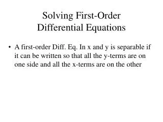
DEFINITION 2.1 Separable Equations A first-order DE of the formdy/dx = g(x)h(y)is said to be separable or to have separable variables. 2.2 Separable Variables • Introduction: Consider dy/dx = f(x, y) = g(x).The DEdy/dx = g(x)(1)can be solved by integration. Integrating both sides to get y = g(x) dx = G(x) + c.eg: dy/dx = 1 + e2x, then y = (1 + e2x)dx = x + ½ e2x + c
Rewrite the above equation as(2)where p(y) =1/h(y).When h(y) = 1, (2) reduces to (1).
If y = (x)is a solution of (2), we must have and(3)But dy = (x) dx, (3)is the same as(4)
Example 1 Solve (1 + x) dy – y dx = 0. Solution:Since dy/y = dx/(1 + x), we haveReplacing by c, gives y = c(1 + x).
Example 2 Solve Solution:We also can rewrite the solution asx2+ y2 = c2,where c2 =2c1Apply the initial condition, 16 + 9 = 25 = c2See Fig2.18.
Losing a Solution • When r is a zero of h(y), then y = r is also a solution of dy/dx = g(x)h(y).However, this solution will not show up after integration. That is a singular solution.
Example 3 Solve dy/dx = y2 – 4. Solution:Rewrite this DE as (5)then
Example 3 (2) Replacing exp(c2)by c andsolving for y, we have(6)If we rewrite the DE as dy/dx = (y + 2)(y – 2),from the previous discussion, we have y = 2is a singular solution.
Example 4 Solve Solution:Rewrite this DE asusing sin2x = 2sin x cos x, then (ey – ye-y) dy = 2sin x dx from integration by parts,ey + ye-y + e-y = -2cos x + c (7)From y(0) =0,we have c = 4 to getey + ye-y + e-y = 4 −2 cos x (8)
Use of Computers • Let G(x, y) = ey + ye-y + e-y + 2 cos x. Using some computer software, we plot the level curves of G(x, y) = c. The resulting graphs are shown in Fig2.19 and Fig2.20.
If we solve dy/dx = xy½, y(0) = 0(9)The resulting graphs are shown in Fig2.21.
DEFINITION 2.2 Linear Equations A first-order DE of the forma1(x)(dy/dx) + a0(x)y = g(x) (1)is said to be a linear equation iny. When g(x) = 0,(1) is said to be homogeneous; otherwise it is nonhomogeneous. 2.3 Linear Equations • Introduction:Linear DEs are friendly to be solved. We can find some smooth methods to deal with.
Standard FormThe standard for of a first-order DE can be written asdy/dx + P(x)y = f(x)(2) • The PropertyDE (2) has the property that its solution is sum of two solutions, y = yc + yp, where yc is a solution of the homogeneous equationdy/dx + P(x)y = 0 (3)and yp is a particular solution of (2).
VerificationNow (3) is also separable. Rewrite (3) as • Solving for y gives
Variation of Parameters • Let yp = u(x) y1(x), where y1(x)is defined as above.We want to find u(x) so that yp is also a solution. Substituting ypinto (2) gives
Since dy1/dx + P(x)y1 = 0, so that y1(du/dx) = f(x) Rearrange the above equation, From the definition of y1(x), we have (4)
Solving Procedures • If (4) is multiplied by (5)then (6)is differentiated (7)we get (8)Dividing (8) by gives (2).
Integrating Factor • We call y1(x) = is an integrating factor and we should only memorize this to solve problems.
Example 1 Solve dy/dx – 3y = 6. Solution:Since P(x)= – 3,we have the integrating factor is then is the same as So e-3xy = -2e-3x + c, a solution is y = -2 + ce-3x, - < x < .
Notes • The DE of example 1 can be written as so that y = –2is a critical point.
General Solutions • Equation (4) is called the general solution on some interval I. Suppose again P and f are continuous on I. Writing (2) as Suppose again Pandfare continuous onI. Writing (2)as y = F(x, y)we identify F(x, y) = – P(x)y + f(x),F/y = –P(x)which are continuous on I.Then we can conclude that there exists one and only one solution of(9)
Example 2 Solve Solution:Dividing both sides by x, we have (10)So, P(x)= –4/x, f(x) = x5ex, P and f are continuous on (0, ).Since x > 0,we write the integrating factor as