Download
1 / 32
320 likes | 479 Views
Chapter 4: Advanced IR Models. 4.1 Probabilistic IR 4.2 Statistical Language Models (LMs) 4.3 Latent-Concept Models 4.3.1 Foundations from Linear Algebra 4.3.2 Latent Semantic Indexing (LSI) 4.3.3 Probabilistic Aspect Model (pLSI). Key Idea of Latent Concept Models. Objective:

E N D
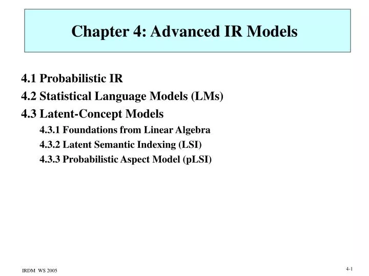
Chapter 4: Advanced IR Models • 4.1 Probabilistic IR • 4.2 Statistical Language Models (LMs) • 4.3 Latent-Concept Models • 4.3.1 Foundations from Linear Algebra • 4.3.2 Latent Semantic Indexing (LSI) • 4.3.3 Probabilistic Aspect Model (pLSI)
Key Idea of Latent Concept Models • Objective: • Transformation of document vectors from • high-dimensional term vector space into • lower-dimensional topic vector space with • exploitation of term correlations • (e.g. „Web“ and „Internet“ frequently occur in together) • implicit differentiation of polysems that exhibit • different term correlations for different meanings • (e.g. „Java“ with „Library“ vs. „Java“ with „Kona Blend“ vs. „Java“ with „Borneo“) mathematically: given: m terms, n docs (usually n > m) and a mn term-document similarity matrix A, needed: largely similarity-preserving mapping of column vectors of A into k-dimensional vector space (k << m) for given k
4.3.1 Foundations from Linear Algebra A set S of vectors is called linearly independent if no x S can be written as a linear combination of other vectors in S. The rankof matrix A is the maximal number of linearly independent row or column vectors. A basis of an nn matrix A is a set S of row or column vectors such that all rows or columns are linear combinations of vectors from S. A set S of n1 vectors is an orthonormal basis if for all x, y S:
Let A be a real-valued nn matrix, x a real-valued n1 vector, and a real-valued scalar. Solutions x and of the equation A x = x are called an Eigenvector and Eigenvalue of A. Eigenvectors of A are vectors whose direction is preserved by the linear transformation described by A. Eigenvalues and Eigenvectors The Eigenvalues of A are the roots (Nullstellen) of the characteristic polynom f() of A: with the determinant (developing the i-th row): where matrix A(ij) is derived from A by removing the i-th row and the j-th column The real-valued nn matrix A is symmetric if aij=aji for all i, j. A is positive definite if for all n1 vectors x 0: xT A x > 0. If A is symmetric then all Eigenvalues of A are A real. If A is symmetric and positive definite then all Eigenvalues are positive.
Illustration of Eigenvectors Matrix describes affine transformation Eigenvector x1 = (0.52 0.85)T for Eigenvalue 1=3.62 Eigenvector x2 = (0.85 -0.52)T for Eigenvalue 2=1.38
Principal Component Analysis (PCA) Spectral Theorem: (PCA, Karhunen-Loewe transform): Let A be a symmetric nn matrix with Eigenvalues 1, ..., n and Eigenvectors x1, ..., xn such that for all i. The Eigenvectors form an orthonormal basis of A. Then the following holds: D = QT A Q, where D is a diagonal matrix with diagonal elements 1, ..., n and Q consists of column vectors x1, ..., xn. often applied to covariance matrix of n-dim. data points
Singular Value Decomposition (SVD) Theorem: Each real-valued mn matrix A with rank r can be decomposed into the form A = U VT with an mr matrix U with orthonormal column vectors, an rr diagonal matrix , and an nr matrix V with orthonormal column vectors. This decomposition is called singular value decomposition and is unique when the elements of or sorted. • Theorem: • In the singular value decomposition A = U VT of matrix A • the matrices U, , and V can be derived as follows: • consists of the singular values of A, • i.e. the positive roots of the Eigenvalues of AT A, • the columns of U are the Eigenvectors of A AT, • the columns of V are the Eigenvectors of AT A.
SVD for Regression Theorem: Let A be an mn matrix with rank r, and let Ak = Uk k VkT, where the kk diagonal matrix k contains the k largest singular values of A and the mk matrix Uk and the nk matrix Vk contain the corresponding Eigenvectors from the SVD of A. Among all mn matrices C with rank at most k Ak is the matrix that minimizes the Frobenius norm y y‘ Example: m=2, n=8, k=1 projection onto x‘ axis minimizes „error“ or maximizes „variance“ in k-dimensional space x‘ x
latent topic t doc j V T U VkT Uk k A doc j 1 1 0 .. ....... 0 .............. .............. ........................ = ........... ........ ...................... ........................ ........ .............. .............. ......... ...................... latent topic t k term i 0 0 r rn rr mn kn kk mr mn mk mapping of m1 vectors into latent-topic space: dj‘Tq‘ = ((kVkT)*j)T q’ scalar-product similarity in latent-topic space: 4.3.2 Latent Semantic Indexing (LSI) [Deerwester et al. 1990]:Applying SVD to Vector Space Model • A is the mn term-document similarity matrix. Then: • U and Uk are the mr and mk term-topic similarity matrices, • V and Vk are the nr and nk document-topic similarity matrices, • AAT and AkAkT are the mm term-term similarity matrices, • ATA and AkTAk are the nn document-document similarity matrices
Indexing and Query Processing • The matrix k VkT corresponds to a „topic index“ and • is stored in a suitable data structure. • Instead of k VkT the simpler index VkT could be used. • Additionally the term-topic mapping Uk must be stored. • A query q (an m1 column vector) in the term vector space • is transformed into query q‘= UkT q (a k1 column vector) • and evaluated in the topic vector space (i.e. Vk) • (e.g. by scalar-product similarity VkT q‘ or cosine similarity) • A new document d (an m1 column vector) is transformed into • d‘ = UkT d (a k 1 column vector) and • appended to the „index“ VkT as an additional column („folding-in“)
m=5 (interface, library, Java, Kona, blend), n=7 VT U Example 1 for Latent Semantic Indexing query q = (0 0 1 0 0)T is transformed into q‘ = UT q = (0.58 0.00)T and evaluated on VT the new document d8 = (1 1 0 0 0)T is transformed into d8‘ = UT d8 = (1.16 0.00)T and appended to VT
Example 2 for Latent Semantic Indexing n=5 documents d1: How to bake bread without recipes d2: The classic art of Viennese Pastry d3: Numerical recipes: the art of scientific computing d4: Breads, pastries, pies and cakes: quantity baking recipes d5: Pastry: a book of best French recipes m=6 terms t1: bak(e,ing) t2: recipe(s) t3: bread t4: cake t5: pastr(y,ies) t6: pie
U VT Example 2 for Latent Semantic Indexing (2)
Example 2 for Latent Semantic Indexing (4) query q: baking bread q = ( 1 0 1 0 0 0 )T transformation into topic space with k=3 q‘ = UkT q = (0.5340 -0.5134 1.0616)T scalar product similarity in topic space with k=3: sim (q, d1) = Vk*1T q‘ 0.86 sim (q, d2) = Vk*2T q -0.12 sim (q, d3) = Vk*3T q‘ -0.24 etc. Folding-in of a new document d6: algorithmic recipes for the computation of pie d6 = ( 0 0.7071 0 0 0 0.7071 )T transformation into topic space with k=3 d6‘ = UkT d6 ( 0.5 -0.28 -0.15 ) d6‘ is appended to VkT as a new column
Construct LSI model (Uk, k, VkT) from • training documents that are available in multiple languages: • consider all language variants of the same document • as a single document and • extract all terms or words for all languages. • Maintain index for further documents by „folding-in“, i.e. • mapping into topic space and appending to VkT. • Queries can now be asked in any language, and the • query results include documents from all languages. Multilingual Retrieval with LSI Example: d1: How to bake bread without recipes. Wie man ohne Rezept Brot backen kann. d2: Pastry: a book of best French recipes. Gebäck: eine Sammlung der besten französischen Rezepte. Terms are e.g. bake, bread, recipe, backen, Brot, Rezept, etc. Documents and terms are mapped into compact topic space.
Towards Self-tuning LSI [Bast et al. 2005] • Project data to its top k eigenvectors (SVD): A Uk k VTk latent concepts (LSI) • This discovers hidden term relations in Uk UkT : • proof / provers: -0.68 • voronoi / diagram: 0.73 • logic / geometry: -0.12 • Central question: which k is the best? proof / provers relatedness voronoi / diagram logic / geometry Assess the shape of the graph, not specific values! dimension dimension dimension • new „dimension-less“ variant of LSI: use 0-1-rounded expansion matrix Uk UkT to expand docs outperforms standard LSI
Summary of LSI • Elegant, mathematically well-founded model • „Automatic learning“ of term correlations • (incl. morphological variants, multilingual corpus) • Implicit thesaurus (by correlations between synonyms) • Implicit discrimination of different meanings of polysems • (by different term correlations) • Improved precision and recall on „closed“ corpora • (e.g. TREC benchmark, financial news, patent databases, etc.) • with empirically best k in the order of 100-200 • In general difficult choice of appropriate k • Computational and storage overhead for very large (sparse) matrices • No convincing results for Web search engines (yet)
economic imports embargo 4.3.3 Probabilistic LSI (pLSI) d and w conditionally independent given z TRADE documents d latent concepts z (aspects) terms w (words)
Relationship of pLSI to LSI P[d|z]· P[z] · P[w|z] VkT Uk k 1 0 .. ....... .............. ...................... ........................ ........ .............. k 0 kn kk mn mk doc probs per concept concept probs term probs per concept • Key difference to LSI: • non-negative matrix decomposition • with L1 normalization • Key difference to LMs: • no generative model for docs • tied to given corpus
Power of Non-negative Matrix Factorization vs. SVD x2 x2 x1 x1 SVD of data matrix A NMF of data matrix A
Expectation-Maximization Method (EM) • Key idea: • when L(, X1, ..., Xn) (where the Xi and are possibly multivariate) • is analytically intractable then • introduce latent (hidden, invisible, missing) random variable(s) Z • such that • the joint distribution J(X1, ..., Xn, Z, ) of the „complete“ data • is tractable (often with Z actually being Z1, ..., Zn) • derive the incomplete-data likelihood L(, X1, ..., Xn) by • integrating (marginalization) J:
EM Procedure Initialization:choose start estimate for (0) Iterate(t=0, 1, …) until convergence: E step (expectation): estimate posterior probability of Z: P[Z | X1, …, Xn, (t)] assuming were known and equal to previous estimate (t), and compute EZ | X1, …, Xn, (t)[log J(X1, …, Xn, Z | )] by integrating over values for Z M step (maximization, MLE step): Estimate (t+1) by maximizing EZ | X1, …, Xn, (t) [log J(X1, …, Xn, Z | )] convergence is guaranteed (because the E step computes a lower bound of the true L function, and the M step yields monotonically non-decreasing likelihood), but may result in local maximum of log-likelihood function
EM at Indexing Time(pLSI Model Fitting) observed data: n(d,w) – absolute frequency of word w in doc d model params: P[z|d], P[w|z] for concepts z, words w, docs d maximize log-likelihood E step: posterior probability of latent variables prob. that occurrence of word w in doc d can be explained by concept z M step: MLE with completed data freq. of w associated with z freq. of d associated with z actual procedure „perturbs“ EM for „smoothing“ (avoidance of overfitting) tempered annealing
EM Details (pLSI Model Fitting) (E) (M1) (M2) or equivalently compute P[z], P[d|z], P[w|z] in M step (see S. Chakrabarti, pp. 110/111)
Folding-in of Queries • keep all estimated parameters of the pLSI model fixed • and treat query as a „new document“ to be explained • find concepts that most likely generate the query (query is the only „document“, and P[w | z] is kept invariant) EM for query parameters
Query Processing Once documents and queries are both represented as probability distributions over k concepts (i.e. k1 vectors with L1 length 1), we can use any convenient vector-space similarity measure (e.g. scalar product or cosine or KL divergence).
Experimental Results: Example Source: Thomas Hofmann, Tutorial at ADFOCS 2004
Experimental Results: Precision VSM: simple tf-based vector space model (no idf) Source: Thomas Hofmann, Tutorial „Machine Learning in Information Retrieval“, presented at Machine Learning Summer School (MLSS) 2004, Berder Island, France
Perplexity measure (reflects generalization potential, as opposed to overfitting): Experimental Results: Perplexity with freq on new data Source: T. Hofmann, Machine Learning 42 (2001)
pLSI Summary • Probabilistic variant of LSI • (non-negative matrix factorization with L1 normalization) • Achieves better experimental results than LSI • Very good on „closed“, thematically specialized corpora, • inappropriate for Web • Computationally expensive (at indexing and querying time) • may use faster clustering for estimating P[d|z] instead of EM • may exploit sparseness of query to speed up folding-in • pLSI does not have a generative model (rather tied to fixed corpus) • LDA model (Latent Dirichlet Allocation) • number of latent concept remains model-selection problem • compute for different k, assess on held-out data, choose best
Latent Semantic Indexing: • Grossman/Frieder Section 2.6 • Manning/Schütze Section 15.4 • M.W. Berry, S.T. Dumais, G.W. O‘Brien: Using Linear Algebra for • Intelligent Information Retrieval, SIAM Review Vol.37 No.4, 1995 • S. Deerwester, S.T. Dumais, G.W. Furnas, T.K. Landauer, R. Harshman: • Indexing by Latent Semantic Analysis, JASIS 41(6), 1990 • H. Bast, D. Majumdar: Why Spectral Retrieval Works, SIGIR 2005 • W.H. Press: Numerical Recipes in C, Cambridge University Press, • 1993, available online at http://www.nr.com/ • G.H. Golub, C.F. Van Loan: Matrix Computations, John Hopkins • University Press, 1996 • pLSI and Other Latent-Concept Models: • Chakrabarti Section 4.4.4 • T. Hofmann: Unsupervised Learning by Probabilistic Latent Semantic Analysis, Machine Learning 42, 2001 • T. Hofmann: Matrix Decomposition Techniques in Machine Learning and • Information Retrieval, Tutorial Slides, ADFOCS 2004 • D. Blei, A. Ng, M. Jordan: Latent Dirichlet Allocation, Journal of Machine • Learning Research 3, 2003 • W. Xu, X. Liu, Y. Gong: Document Clustering based on Non-negative • Matrix Factorization, SIGIR 2003 Additional Literature for Chapter 4