Download
1 / 12
420 likes | 1.78k Views
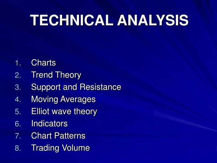
TECHNICAL ANALYSIS. Charts Trend Theory Support and Resistance Moving Averages Elliot wave theory Indicators Chart Patterns Trading Volume. Chart Types : Line charts Bar charts (open-high-low-close bars) Candlestick charts (also, volume-adjusted bar size)

E N D
TECHNICAL ANALYSIS Charts Trend Theory Support and Resistance Moving Averages Elliot wave theory Indicators Chart Patterns Trading Volume
Chart Types: • Line charts • Bar charts (open-high-low-close bars) • Candlestick charts (also, volume-adjusted bar size) • Point and Figure Charts (X up, O down) Trend Theory: A local maximum is called High, and a local minimum is called Low. Uptrend = higher High’s and higher Low’s Downtrend = lower High’s and lower Low’s “Trend is your friend”
Trendlines: Uptrendline: connect consecutive Low’s once uptrend is confirmed. Downtrendline: connect consecutive High’s once downtrendis confirmed. Channel Lines: parallels of trendlines. Support lines: connect consecutive Low’s when no uptrend is evident. Resistance lines: connect consecutive High’s when no downtrend is evident.
SUPPORT: A level where buyers are expected to dominate sellers. RESISTANCE: A level where sellers are expected to dominate buyers. What acts as S or R ? • Previous H’s and L’s • Uptrendlines act as S, Downtrendlines act as R • Upchannellines act as R, Downchannellines act as S • S and R lines • Moving Averages • Fibonacci Retracement Levels
MOVING AVERAGES Simple, Exponential, Weighted. Use simple. Moving Average Crossover Rules: Buy when the price (which is MA(1)) or MA(s) crosses the MA(l) up from below. Sell when the price (which is MA(1)) or MA(s) crosses the MA(l) down from above.
A strategic question: Can you predict whether a S or R will hold or be breached? Yes, to some extent. The significance of a S or R depends on: 1) how many times it has been tested and has held 2) for how long it has held 3) slope 4) chart frequency The strength of a S or R depends on: 1) previous move before the test 2) type, slope 3) chart frequency
INDICATORS Derived from the price, using complex mathematical calculations. Help visual decision making. MACD: practically, MACD(l,s,t) = EMA(s)−EMA(l) where the trigger line is a t-period mov.avg. of the MACD, Stochastic Oscillator: %K = (C – Ln) / (Hn−Ln) %D = MA(%K) %D is the t-period mov.avg. of %D and acts as the trigger line
CHART PATTERNS Reversal Patterns • Head-and-Shoulder and Inverse H-S • Double top and double bottom • Diamond Consolidation Patterns • Ascending Triangle, Descending Triangle • Flag, Pennant • Rectangle • Rising Wedge, Falling Wedge
The Sources of TA’s predictive power • Asymmetric private information • (short-lag positive and long-lag negative) autocorrelation in macroeconomic data • Gradual revision of beliefs Underreaction and overreaction 4) Self-fulfilling prophecy
How to benefit from TA? * In social sciences there are no absolute truths. So, the efficacy of TA is not stable. * For an experienced professional trader, it is at least: a tool to read the mind of others, to mechanize buy-sell decisions, to detect asymmetric information. A smart-technical system can make net money on the average (combine it with “buy-low-sell-high” principle). TA is an inevitable part of full toolkit. * For an amateur investor: it is probably a cheaper and usually better guide than most alternative guides (provided that it is employed properly recalling its limitations). * For a corporate financial manager, it is a complementary in exploiting financial information or maximizing market value of your company.
ACADEMIC WORK ON RETURN PREDICTABILITY Two Tasks in Investing: Timing and Stock Selection Strategy Direction: Momentum Strategies:Positive Feedback Trading Contrarian Strategies: Negative Feedback Trading Autocorrelation in Returns: Rt = 0 + 1Rt-1 + 2Rt-2 + 3Rt-3 + …+et
History of Academic Thinking on Predictability in Financial Markets 1870-1920: Public participation in stock markets begins, TA develops even before Financial analysis. 1930-50: The idea of efficient (unpredictable) markets emerges. 1952: Markowitz’ portfolio theory 1964: CAPM (Sharpe, Merton) 1970: Efficient Markets Theory (Fama) 1970-1980’s: Efficient Markets Theory firmly dominates academic thinking. 1985: the first studies on Behavioral Finance (1979 Kahneman) 1990’s: Rain of evidence against efficient markets Hot debate between proponents and opponents of EMT 2000’s: Behavioral Finance gains widespread acceptance However, markets are more unpredictable. 2008: New Paradigm: Reflexivity