Download
1 / 24
250 likes | 295 Views
Learn the mathematical analysis of queues and waiting times in stochastic systems, essential for industries facing demand fluctuations. Explore examples, such as ER operations, and grasp the importance of queuing analysis for capacity optimization and productivity gains. Understand real-world queuing systems in commercial, transportation, business-internal, and social service sectors. Delve into the components of a basic queuing process, from input source to queue configuration, and discover the advantages of multiple vs. single customer queue configurations.

E N D
Queuing System Dr. Adil Yousif Lecture 2
What is Queuing Theory? • Mathematical analysis of queues and waiting times in stochastic systems. • Used extensively to analyze production and service processes exhibiting random variability in market demand (arrival times) and service times. • Queues arise when the short term demand for service exceeds the capacity • Most often caused by random variation in service times and the times between customer arrivals. • If long term demand for service > capacity the queue will explode!
Why is Queuing Analysis Important? • Capacity problems are very common in industry and one of the main drivers of process redesign • Need to balance the cost of increased capacity against the gains of increased productivity and service • Queuing and waiting time analysis is particularly important in service systems • Large costs of waiting and of lost sales due to waiting Prototype Example – ER at County Hospital • Patients arrive by ambulance or by their own accord • One doctor is always on duty • More and more patients seeks help longer waiting times • Question: Should another MD position be instated?
Total cost Cost Cost of service Cost of waiting Process capacity A Cost/Capacity Tradeoff Model
Examples of Real World Queuing Systems? • Commercial Queuing Systems • Commercial organizations serving external customers • Ex. Dentist, bank, ATM, gas stations, plumber, garage … • Transportation service systems • Vehicles are customers or servers • Ex. Vehicles waiting at toll stations and traffic lights, trucks or ships waiting to be loaded, taxi cabs, fire engines, elevators, buses … • Business-internal service systems • Customers receiving service are internal to the organization providing the service • Ex. Inspection stations, conveyor belts, computer support … • Social service systems • Ex. Judicial process, the ER at a hospital, waiting lists for organ transplants or student dorm rooms …
Arrival event Schedule the next arrival event Yes Is the server busy? No Add 1to the number in queue Set delay = 0 for this customer and gather statistics Write error message and stop simulation Yes Is the queue Full? Add 1 to thenumber of customers delayed No Store time of arrival of this customer Make the server busy Schedule a departure event for this customer Return Flowchart for arrival routine, queuing model
Departure event Yes Is the queue empty? No Make the server idle Subtract 1 from the number in queue Eliminate departure event from consideration Compute delay of customer entering service and gather statistics Add 1 to the number of customers delayed Schedule a departure event for this customer Move each customer in queue (if any) up one place Return Flowchart for departure routine,queueing model
Components of a Basic Queuing Process Input Source The Queuing System Served Jobs Service Mechanism Calling Population Jobs Queue leave the system Queue Discipline Arrival Process Service Process Queue Configuration
Components of a Basic Queuing Process (II) • The calling population • The population from which customers/jobs originate • The size can be finite or infinite (the latter is most common) • Can be homogeneous (only one type of customers/ jobs) or heterogeneous (several different kinds of customers/jobs) • The Arrival Process • Determines how, when and where customer/jobs arrive to the system • Important characteristic is the customers’/jobs’ inter-arrival times • To correctly specify the arrival process requires data collection of interarrival times and statistical analysis.
Components of a Basic Queuing Process (III) • The queue configuration • Specifies the number of queues • Single or multiple lines to a number of service stations • Their location • Their effect on customer behavior • Balking and reneging • Their maximum size (# of jobs the queue can hold) • Distinction between infinite and finite capacity
Multiple Queues Single Queue Servers Servers Example – Two Queue Configurations
The service provided can be differentiated Ex. Supermarket express lanes Labor specialization possible Customer has more flexibility Balking behavior may be deterred Several medium-length lines are less intimidating than one very long line Guarantees fairness FIFO applied to all arrivals No customer anxiety regarding choice of queue Avoids “cutting in” problems The most efficient set up for minimizing time in the queue Jockeying (line switching) is avoided Multiple v.s. Single Customer Queue Configuration Multiple Line Advantages Single Line Advantages
Components of a Basic Queuing Process (IV) • The Service Mechanism • Can involve one or several service facilities with one or several parallel service channels (servers) - Specification is required • The service provided by a server is characterized by its service time • Specification is required and typically involves data gathering and statistical analysis. • Most analytical queuing models are based on the assumption of exponentially distributed service times, with some generalizations. • The queue discipline • Specifies the order by which jobs in the queue are being served. • Most commonly used principle is FIFO. • Other rules are, for example, LIFO, SPT, EDD… • Can entail prioritization based on customer type.
Mitigating Effects of Long Queues • Concealing the queue from arriving customers • Ex. Restaurants divert people to the bar or use pagers, amusement parks require people to buy tickets outside the park, banks broadcast news on TV at various stations along the queue, casinos snake night club queues through slot machine areas. • Use the customer as a resource • Ex. Patient filling out medical history form while waiting for physician • Making the customer’s wait comfortable and distracting their attention • Ex. Complementary drinks at restaurants, computer games, internet stations, food courts, shops, etc. at airports • Explain reason for the wait • Provide pessimistic estimates of the remaining wait time • Wait seems shorter if a time estimate is given. • Be fair and open about the queuing disciplines used
A Commonly Seen Queuing Model (I) The Queuing System The Service Facility C S = Server C S • • • C S The Queue Customers (C) C C C … C Customer =C
A Commonly Seen Queuing Model (II) • Service times as well as interarrival times are assumed independent and identically distributed • If not otherwise specified • Commonly used notation principle: A/B/C • A = The interarrival time distribution • B = The service time distribution • C = The number of parallel servers • Commonly used distributions • M = Markovian (exponential) - Memoryless • D = Deterministic distribution • G = General distribution • Example: M/M/c • Queuing system with exponentially distributed service and inter-arrival times and c servers
The Exponential Distribution and Queuing • The most commonly used queuing models are based on the assumption of exponentially distributed service times and interarrival times. Definition: A stochastic (or random) variable Texp( ), i.e., is exponentially distributed with parameter , if its frequency function is: The Cumulative Distribution Function is: The mean = E[T] = 1/ The Variance = Var[T] = 1/ 2
The Exponential Distribution fT(t) Probability density t Mean= E[T]=1/ Time between arrivals
Properties of the Exp-distribution (IV) • Relationship to the Poisson distribution and the Poisson Process Let X(t) be the number of events occurring in the interval [0,t]. If the time between consecutive events is T and Texp() • X(t)Po(t) {X(t), t0} constitutes a Poisson Process
X(t)=# Calls t Stochastic Processes in Continuous Time • Definition: A stochastic process in continuous time is a family {X(t)} of stochastic variables defined over a continuous set of t-values. • Example: The number of phone calls connected through a switch board • Definition:A stochastic process{X(t)} is said to have independent increments if for all disjoint intervals (ti, ti+hi) the differences Xi(ti+hi)Xi(ti) are mutually independent.
The Poisson Process • The standard assumption in many queuing models is that the arrival process is Poisson Two equivalent definitions of the Poisson Process • The times between arrivals are independent, identically distributed and exponential • X(t) is a Poisson process with arrival rate .
Terminology and Notation • The state of the system = the number of customers in the system • Queue length = (The state of the system) – (number of customers being served) N(t)= Number of customers/jobs in the system at time t Pn(t)= The probability that at time t, there are n customers/jobs in the system. n= Average arrival intensity (= # arrivals per time unit) at n customers/jobs in the system n= Average service intensity for the system when there are n customers/jobs in it. (Note, the total service intensity for all occupied servers) = The utilization factor for the service facility. (= The expected fraction of the time that the service facility is being used)
Example – Service Utilization Factor • Consider an M/M/1 queue with arrival rate = and service intensity = • = Expected capacity demand per time unit • = Expected capacity per time unit • • Similarly if there are c servers in parallel, i.e., an M/M/c system but the expected capacity per time unit is then c* •