Download
1 / 47
500 likes | 792 Views
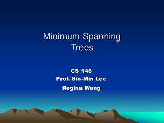
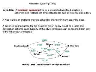
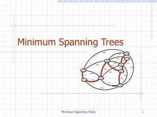
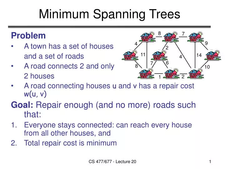
8. 7. b. c. d. 9. 4. 2. a. e. i. 11. 14. 4. 6. 7. 8. 10. h. g. f. 2. 1. Minimum Spanning Trees. Problem A town has a set of houses and a set of roads A road connects 2 and only 2 houses A road connecting houses u and v has a repair cost w(u, v)

E N D
8 7 b c d 9 4 2 a e i 11 14 4 6 7 8 10 h g f 2 1 Minimum Spanning Trees Problem • A town has a set of houses and a set of roads • A road connects 2 and only 2 houses • A road connecting houses u and v has a repair cost w(u, v) Goal: Repair enough (and no more) roads such that: • Everyone stays connected: can reach every house from all other houses, and • Total repair cost is minimum CS 477/677 - Lecture 20
8 7 b c d 9 4 2 a e i 11 14 4 6 7 8 10 h g f 2 1 Minimum Spanning Trees • A connected, undirected graph: • Vertices = houses, Edges = roads • A weight w(u, v) on each edge (u, v) E Find T E such that: • T connects all vertices • w(T) = Σ(u,v)T w(u, v) is minimized CS 477/677 - Lecture 20
8 7 b c d 9 4 2 a e i 11 14 4 6 7 8 10 g g f 2 1 Minimum Spanning Trees • T forms a tree = spanning tree • A spanning tree whose weight is minimum over all spanning trees is called a minimum spanning tree, or MST. CS 477/677 - Lecture 20
8 7 b c d 9 4 2 a e i 11 14 4 6 7 8 10 h g f 2 1 Properties of Minimum Spanning Trees • Minimum spanning trees are not unique • Can replace (b, c) with (a, h) to obtain a different spanning tree with the same cost • MST have no cycles • We can take out an edge of a cycle, and still have the vertices connected while reducing the cost • # of edges in a MST: • |V| - 1 CS 477/677 - Lecture 20
8 7 b c d 9 4 2 a e i 11 14 4 6 7 8 10 h g f 2 1 Growing a MST Minimum-spanning-tree problem: find a MST for a connected, undirected graph, with a weight function associated with its edges A generic solution: • Build a set A of edges (initially empty) • Incrementally add edges to A such that they would belong to a MST • An edge (u, v) is safe for A if and only if A {(u, v)} is also a subset of some MST We will add only safe edges CS 477/677 - Lecture 20
8 7 b c d 9 4 2 a e i 11 14 4 6 7 8 10 h g f 2 1 Generic MST algorithm • A ← • while A is not a spanning tree • do find an edge (u, v) that is safe for A • A ← A {(u, v)} • return A • How do we find safe edges? CS 477/677 - Lecture 20
We would add edge (c, f) 8 7 b c d 9 4 2 a e i 11 14 4 6 7 8 10 h g f 2 1 The Algorithm of Kruskal • Start with each vertex being its own component • Repeatedly merge two components into one by choosing the light edge that connects them • Scan the set of edges in monotonically increasing order by weight • Uses a disjoint-set data structure to determine whether an edge connects vertices in different components CS 477/677 - Lecture 20
Operations on Disjoint Data Sets • MAKE-SET(u) – creates a new set whose only member is u • FIND-SET(u) – returns a representative element from the set that contains u • May be any of the elements of the set that has a particular property • E.g.: Su = {r, s, t, u}, the property is that the element be the first one alphabetically FIND-SET(u) = r FIND-SET(s) = r • FIND-SET has to return the same value for a given set CS 477/677 - Lecture 20
Operations on Disjoint Data Sets • UNION(u, v) – unites the dynamic sets that contain u and v, say Su and Sv • E.g.: Su = {r, s, t, u}, Sv = {v, x, y} UNION (u, v) = {r, s, t, u, v, x, y} CS 477/677 - Lecture 20
KRUSKAL(V, E, w) • A ← • for each vertex v V • do MAKE-SET(v) • sort E into non-decreasing order by weight w • for each (u, v) taken from the sorted list • do if FIND-SET(u) FIND-SET(v) • then A ← A {(u, v)} • UNION(u, v) • return A Running time: O(E lgV) – dependent on the implementation of the disjoint-set data structure CS 477/677 - Lecture 20
8 7 b c d 9 4 2 a e i 11 14 4 6 7 8 10 h g f 2 1 Example • Add (h, g) • Add (c, i) • Add (g, f) • Add (a, b) • Add (c, f) • Ignore (i, g) • Add (c, d) • Ignore (i, h) • Add (a, h) • Ignore (b, c) • Add (d, e) • Ignore (e, f) • Ignore (b, h) • Ignore (d, f) {g, h}, {a}, {b}, {c}, {d}, {e}, {f}, {i} {g, h}, {c, i}, {a}, {b}, {d}, {e}, {f} {g, h, f}, {c, i}, {a}, {b}, {d}, {e} {g, h, f}, {c, i}, {a, b}, {d}, {e} {g, h, f, c, i}, {a, b}, {d}, {e} {g, h, f, c, i}, {a, b}, {d}, {e} {g, h, f, c, i, d}, {a, b}, {e} {g, h, f, c, i, d}, {a, b}, {e} {g, h, f, c, i, d, a, b}, {e} {g, h, f, c, i, d, a, b}, {e} {g, h, f, c, i, d, a, b, e} {g, h, f, c, i, d, a, b, e} {g, h, f, c, i, d, a, b, e} {g, h, f, c, i, d, a, b, e} 1: (h, g) 2: (c, i), (g, f) 4: (a, b), (c, f) 6: (i, g) 7: (c, d), (i, h) 8: (a, h), (b, c) 9: (d, e) 10: (e, f) 11: (b, h) 14: (d, f) {a}, {b}, {c}, {d}, {e}, {f}, {g}, {h},{i} CS 477/677 - Lecture 20
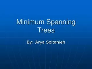
8 7 b c d 9 4 2 a e i 11 14 4 6 7 8 10 h g f 2 1 The algorithm of Prim • The edges in set A always form a single tree • Starts from an arbitrary “root”: VA = {a} • At each step: • Find a light edge crossing cut (VA, V - VA) • Add this edge to A • Repeat until the tree spans all vertices • Greedy strategy • At each step the edge added contributes the minimum amount possible to the weight of the tree CS 477/677 - Lecture 20
8 7 b c d 9 4 2 a e i 11 14 4 6 7 8 10 h g f 2 1 How to Find Light Edges Quickly? Use a priority queue Q: • Contains all vertices not yet included in the tree (V – VA) • V = {a}, Q = {b, c, d, e, f, g, h, i} • With each vertex we associate a key: key[v] = minimum weight of any edge (u, v) connecting v to a vertex in the tree • Key of v is if v is not adjacent to any vertices in VA • After adding a new node to VA we update the weights of all the nodes adjacent to it • We added node a key[b] = 4, key[h] = 8 CS 477/677 - Lecture 20
8 7 b c d 9 4 2 a e i 11 14 4 6 7 8 10 h g f 2 1 PRIM(V, E, w, r) • Q ← • for each u V • do key[u] ← ∞ • π[u] ← NIL • INSERT(Q, u) • DECREASE-KEY(Q, r, 0) • while Q • do u ← EXTRACT-MIN(Q) • for each vAdj[u] • do if v Q and w(u, v) < key[v] • then π[v] ← u • DECREASE-KEY(Q, v, w(u, v)) 0 0 Q = {a, b, c, d, e, f, g, h, i} VA = Extract-MIN(Q) a CS 477/677 - Lecture 20
4 8 8 8 7 7 b b c c d d 9 9 4 4 2 2 a a e e i i 11 11 14 14 4 4 6 6 7 7 8 8 10 10 h h g g f f 2 2 1 1 Example 0 Q = {a, b, c, d, e, f, g, h, i} VA = Extract-MIN(Q) a key [b] = 4 [b] = a key [h] = 8 [h] = a 4 8 Q = {b, c, d, e, f, g, h, i} VA = {a} Extract-MIN(Q) b CS 477/677 - Lecture 20
4 8 8 8 7 7 b b c c d d 8 4 9 9 4 4 2 2 a a e e i i 11 11 14 14 4 4 6 6 7 7 8 8 10 10 h h g g f f 2 2 1 1 8 Example key [c] = 8 [c] = b key [h] = 8 [h] = a - unchanged 8 8 Q = {c, d, e, f, g, h, i} VA = {a, b} Extract-MIN(Q) c 8 key [d] = 7 [d] = c key [f] = 4 [f] = c key [i] = 2 [i] = c 7 4 8 2 Q = {d, e, f, g, h, i} VA = {a, b, c} Extract-MIN(Q) i 7 2 4 CS 477/677 - Lecture 20
8 8 7 7 b b c c d d 8 4 7 8 4 7 9 9 4 4 2 2 a a e e i i 11 11 14 14 4 4 2 2 6 6 7 7 8 8 10 10 h h g g f f 2 2 1 1 4 8 4 6 7 Example key [h] = 7 [h] = i key [g] = 6 [g] = i 7 4 8 Q = {d, e, f, g, h} VA = {a, b, c, i} Extract-MIN(Q) f key [g] = 2 [g] = f key [d] = 7 [d] = c unchanged key [e] = 10 [e] = f 7 10 2 8 Q = {d, e, g, h} VA = {a, b, c, i, f} Extract-MIN(Q) g 6 7 10 2 CS 477/677 - Lecture 20
8 8 7 7 b b c c d d 8 8 4 4 7 7 9 9 4 4 2 2 a a e e i i 11 11 14 14 4 4 10 10 2 2 6 6 7 7 8 8 10 10 h h g g f f 2 2 1 1 4 4 2 2 7 1 Example key [h] = 1 [h] = g 7 10 1 Q = {d, e, h} VA = {a, b, c, i, f, g} Extract-MIN(Q) h 7 10 Q = {d, e} VA = {a, b, c, i, f, g, h} Extract-MIN(Q) d 1 CS 477/677 - Lecture 20
8 7 b c d 8 4 7 9 4 2 a e i 11 14 4 10 2 6 7 8 10 h g f 2 1 4 2 1 Example key [e] = 9 [e] = f 9 Q = {e} VA = {a, b, c, i, f, g, h, d} Extract-MIN(Q) e Q = VA = {a, b, c, i, f, g, h, d, e} 9 CS 477/677 - Lecture 20
PRIM(V, E, w, r) Total time: O(VlgV + ElgV) = O(ElgV) • Q ← • for each u V • do key[u] ← ∞ • π[u] ← NIL • INSERT(Q, u) • DECREASE-KEY(Q, r, 0) ► key[r] ← 0 • while Q • do u ← EXTRACT-MIN(Q) • for each vAdj[u] • do if v Q and w(u, v) < key[v] • then π[v] ← u • DECREASE-KEY(Q, v, w(u, v)) O(V) if Q is implemented as a min-heap Min-heap operations: O(VlgV) Executed |V| times Takes O(lgV) Executed O(E) times O(ElgV) Constant Takes O(lgV) CS 477/677 - Lecture 20
Shortest Path Problems • How can we find the shortest route between two points on a map? • Model the problem as a graph problem: • Road map is a weighted graph: vertices = cities edges = road segments between cities edge weights = road distances • Goal: find a shortest path between two vertices (cities) CS 477/677 - Lecture 20
t x 6 3 9 3 4 1 2 0 s 2 7 p 3 5 5 11 6 y z Shortest Path Problems • Input: • Directed graph G = (V, E) • Weight function w : E → R • Weight of path p = v0, v1, . . . , vk • Shortest-path weight from u to v: δ(u, v) = min w(p) : u v if there exists a path from u to v ∞ otherwise • Shortest path u to v is any path p such that w(p) = δ(u, v) CS 477/677 - Lecture 20
Variants of Shortest Paths • Single-source shortest path • G = (V, E) find a shortest path from a given source vertex s to each vertex v V • Single-destination shortest path • Find a shortest path to a given destination vertex tfrom each vertex v • Reverse the direction of each edge single-source • Single-pair shortest path • Find a shortest path from u to v for given vertices u and v • Solve the single-source problem • All-pairs shortest-paths • Find a shortest path from u to v for every pair of vertices u and v CS 477/677 - Lecture 20
p1i pij pjk Optimal Substructure of Shortest Paths Given: • A weighted, directed graph G = (V, E) • A weight function w: E R, • A shortest path p = v1, v2, . . . , vk from v1 to vk • A subpath of p: pij = vi, vi+1, . . . , vj, with 1 i j k Then: pijis a shortest path from vito vj Proof: p = v1 vi vj vk w(p) = w(p1i) + w(pij) + w(pjk) Assume pij’ from vi to vj with w(pij’) < w(pij) w(p’) = w(p1i) + w(pij’) + w(pjk) < w(p)contradiction! vj pjk pij v1 p1i pij’ vk vi CS 477/677 - Lecture 20
a b -4 3 -1 4 3 c g d 6 8 5 0 - 5 11 s -3 y 2 7 3 - - -6 e f Negative-Weight Edges What if we have negative-weight edges? • s a: only one path (s, a) = w(s, a) = 3 • s b: only one path (s, b) = w(s, a) + w(a, b) = -1 • s c: infinitely many paths s, c, s, c, d, c, s, c, d, c, d, c cycle has positive weight (6 - 3 = 3) s, c is shortest path with weight (s, b) = w(s, c) = 5 CS 477/677 - Lecture 20
a b -4 3 -1 4 3 c g d 6 8 5 0 - 5 11 s -3 y 2 7 3 - - -6 e f h i 2 3 -8 j Negative-Weight Edges • s e: infinitely many paths: • s, e, s, e, f, e, s, e, f, e, f, e • cycle e, f, e has negative weight: 3 + (- 6) = -3 • can find paths from s to e with arbitrarily large negative weights • (s, e) = - no shortest path exists between s and e • Similarly: (s, f) = - , (s, g) = - h, i, j not reachable from s (s, h) = (s, i) =(s, j) = CS 477/677 - Lecture 20
a b -4 4 3 c g d 6 8 5 0 s -3 y 2 7 3 -6 e f Negative-Weight Edges • Negative-weight edges may form negative-weight cycles • If such cycles are reachable from the source: (s, v) is not properly defined • Keep going around the cycle, and get w(s, v) = - for all v on the cycle CS 477/677 - Lecture 20
Cycles • Can shortest paths contain cycles? • Negative-weight cycles • Positive-weight cycles: • By removing the cycle we can get a shorter path • Zero-weight cycles • No reason to use them • Can remove them to obtain a path with similar weight • We will assume that when we are finding shortest paths, the paths will have no cycles No! No! CS 477/677 - Lecture 20
t x 6 3 9 3 4 1 2 0 s 2 7 3 5 5 11 6 y z Shortest-Path Representation For each vertex v V: • d[v] = δ(s, v): a shortest-path estimate • Initially, d[v]=∞ • Reduces as algorithms progress • [v] = predecessor of v on a shortest path from s • If no predecessor, [v] = NIL • induces a tree—shortest-path tree • Shortest paths & shortest path trees are not unique CS 477/677 - Lecture 20
Initialization Alg.: INITIALIZE-SINGLE-SOURCE(V, s) • for each v V • do d[v] ← • [v] ← NIL • d[s] ← 0 • All the shortest-paths algorithms start with INITIALIZE-SINGLE-SOURCE CS 477/677 - Lecture 20
u u u u v v v v s s 2 2 2 2 5 5 5 5 9 6 6 7 Relaxation • Relaxing an edge (u, v) = testing whether we can improve the shortest path to v found so far by going through u If d[v] > d[u] + w(u, v) we can improve the shortest path to v update d[v] and [v] • After relaxation: • d[v] d[u] + w(u, v) RELAX(u, v, w) RELAX(u, v, w) CS 477/677 - Lecture 20
RELAX(u, v, w) • if d[v] > d[u] + w(u, v) • then d[v] ← d[u] + w(u, v) • [v] ← u • All the single-source shortest-paths algorithms • start by calling INIT-SINGLE-SOURCE • then relax edges • The algorithms differ in the order and how many times they relax each edge CS 477/677 - Lecture 20
Bellman-Ford Algorithm • Single-source shortest paths problem • Computes d[v] and [v] for all v V • Allows negative edge weights • Returns: • TRUE if no negative-weight cycles are reachable from the source s • FALSE otherwise no solution exists • Idea: • Traverse all the edges |V – 1| times, every time performing a relaxation step of each edge CS 477/677 - Lecture 20
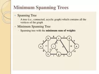
t t x x 5 5 -2 -2 6 6 -3 -3 8 8 7 7 0 0 s s -4 -4 2 2 7 7 9 9 y y z z BELLMAN-FORD(V, E, w, s) • INITIALIZE-SINGLE-SOURCE(V, s) • for i ← 1 to |V| - 1 • do for each edge (u, v) E • do RELAX(u, v, w) • for each edge (u, v) E • do if d[v] > d[u] + w(u, v) • then return FALSE • return TRUE 6 7 E: (t, x), (t, y), (t, z), (x, t), (y, x), (y, z), (z, x), (z, s), (s, t), (s, y) CS 477/677 - Lecture 20
t t t t x x x x 5 5 5 5 6 6 6 6 -2 -2 -2 -2 6 6 6 6 -3 -3 -3 -3 8 8 8 8 7 7 7 7 0 0 0 0 s s s s -4 -4 -4 -4 2 2 2 2 7 7 7 7 7 7 7 7 9 9 9 9 y y y y z z z z 4 4 11 11 2 2 2 Example (t, x), (t, y), (t, z), (x, t), (y, x), (y, z), (z, x), (z, s), (s, t), (s, y) Pass 1 Pass 2 4 11 2 Pass 3 Pass 4 2 -2 CS 477/677 - Lecture 20
s s s b b b 2 2 2 -3 0 0 2 3 3 3 -8 -8 -8 5 c c c Detecting Negative Cycles • for each edge (u, v) E • do if d[v] > d[u] + w(u, v) • then return FALSE • return TRUE Look at edge (s, b): d[b] = -1 d[s] + w(s, b) = -4 d[b] > d[s] + w(s, b) -6 -1 -3 2 2 5 CS 477/677 - Lecture 20
BELLMAN-FORD(V, E, w, s) • INITIALIZE-SINGLE-SOURCE(V, s) • for i ← 1 to |V| - 1 • do for each edge (u, v) E • do RELAX(u, v, w) • for each edge (u, v) E • do if d[v] > d[u] + w(u, v) • then return FALSE • return TRUE Running time: O(VE) (V) O(V) O(E) O(E) CS 477/677 - Lecture 20
u u v v s s 2 2 5 5 7 6 Shortest Path Properties • Triangle inequality For all (u, v) E, we have: δ(s, v) ≤ δ(s, u) + w(u, v) • If u is on the shortest path to v we have the equality sign CS 477/677 - Lecture 20
v v x x 5 5 6 6 -2 -2 6 6 -3 -3 8 8 7 7 0 0 s s -4 -4 2 2 7 7 2 7 7 4 11 9 9 y y z z 4 11 2 2 Shortest Path Properties • Upper-bound property We always have d[v] ≥ δ(s, v) for all v. Once d[v] = δ(s, v), it never changes. • The estimate never goes up – relaxation only lowers the estimate Relax (x, v) CS 477/677 - Lecture 20
a b -4 3 -1 4 3 c g d 6 8 5 0 - 5 11 s -3 y 2 7 3 - - -6 e f h i 2 3 -8 j Shortest Path Properties • No-path property If there is no path from s to v then d[v] = ∞ always. • δ(s, h) = ∞ and d[h] ≥ δ(s, h) d[h] = ∞ h, i, j not reachable from s (s, h) = (s, i) =(s, j) = CS 477/677 - Lecture 20
Shortest Path Properties • Convergence property If s u → v is a shortest path, and if d[u] = δ(s, u) at any time prior to relaxing edge (u, v), then d[v] = δ(s, v) at all times afterward. • If d[v] > δ(s, v) after relaxation: • d[v] = d[u] + w(u, v) • d[v] = 5 + 2 = 7 • Otherwise, the value remains unchanged, because it must have been the shortest path value u v 2 6 5 8 11 5 0 s 4 4 7 CS 477/677 - Lecture 20
Shortest Path Properties • Path relaxation property Let p = v0, v1, . . . , vk be a shortest path from s = v0 to vk. If we relax, in order, (v0, v1), (v1, v2), . . . , (vk-1, vk), even intermixed with other relaxations, then d[vk ] = δ(s, vk). v1 v2 2 d[v2] = δ(s, v2) 6 v4 11 7 5 14 5 3 v3 d[v1] = δ(s, v1) 4 d[v4] = δ(s, v4) 0 s 11 d[v3] = δ(s, v3) CS 477/677 - Lecture 20
u v 2 6 11 5 y 4 4 x Single-Source Shortest Paths in DAGs • Given a weighted DAG: G = (V, E) – solve the shortest path problem • Idea: • Topologically sort the vertices of the graph • Relax the edges according to the order given by the topological sort • for each vertex, we relax each edge that starts from that vertex • Are shortest-paths well defined in a DAG? • Yes, (negative-weight) cycles cannot exist CS 477/677 - Lecture 20
Dijkstra’s Algorithm • Single-source shortest path problem: • No negative-weight edges: w(u, v) > 0 (u, v) E • Maintains two sets of vertices: • S = vertices whose final shortest-path weights have already been determined • Q = vertices in V – S: min-priority queue • Keys in Q are estimates of shortest-path weights (d[v]) • Repeatedly select a vertex u V – S, with the minimum shortest-path estimate d[v] CS 477/677 - Lecture 20
t t x x 1 1 9 9 10 10 2 2 4 4 3 3 6 6 0 0 s s 7 7 5 5 10 2 2 y y z z 5 Dijkstra (G, w, s) • INITIALIZE-SINGLE-SOURCE(V, s) • S ← • Q ← V[G] • while Q • dou ← EXTRACT-MIN(Q) • S ← S {u} • for each vertex v Adj[u] • do RELAX(u, v, w) CS 477/677 - Lecture 20
t t t t x x x x 1 1 1 1 8 8 8 10 13 14 9 8 14 13 9 9 9 9 10 10 10 10 2 2 2 2 4 4 4 4 3 3 3 3 6 6 6 6 0 0 0 0 s s s s 7 7 7 7 5 5 5 5 5 5 5 5 7 7 7 7 2 2 2 2 y y y y z z z z 9 Example CS 477/677 - Lecture 20
Dijkstra (G, w, s) (V) • INITIALIZE-SINGLE-SOURCE(V, s) • S ← • Q ← V[G] • while Q • dou ← EXTRACT-MIN(Q) • S ← S {u} • for each vertex v Adj[u] • do RELAX(u, v, w) Running time: O(VlgV + ElgV) = O(ElgV) O(V) build min-heap Executed O(V) times O(lgV) O(E) times; O(lgV) CS 477/677 - Lecture 20