Download
1 / 6
60 likes | 66 Views
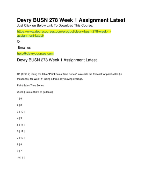
Just Click on Below Link To Download This Course:<br><br>https://www.devrycoursehelp.com/product/devry-busn-278-week-1-assignment-latest/<br><br>Devry BUSN 278 Week 1 Assignment Latest<br> <br>Q1 (TCO 2) Using the table u201cPaint Sales Time Seriesu201d, calculate the forecast for paint sales (in thousands) for Week 11 using a three day moving average.<br>Paint Sales Time Series |<br>Week | Sales (000u2019s of gallons) |<br>1 | 6 |<br>

E N D
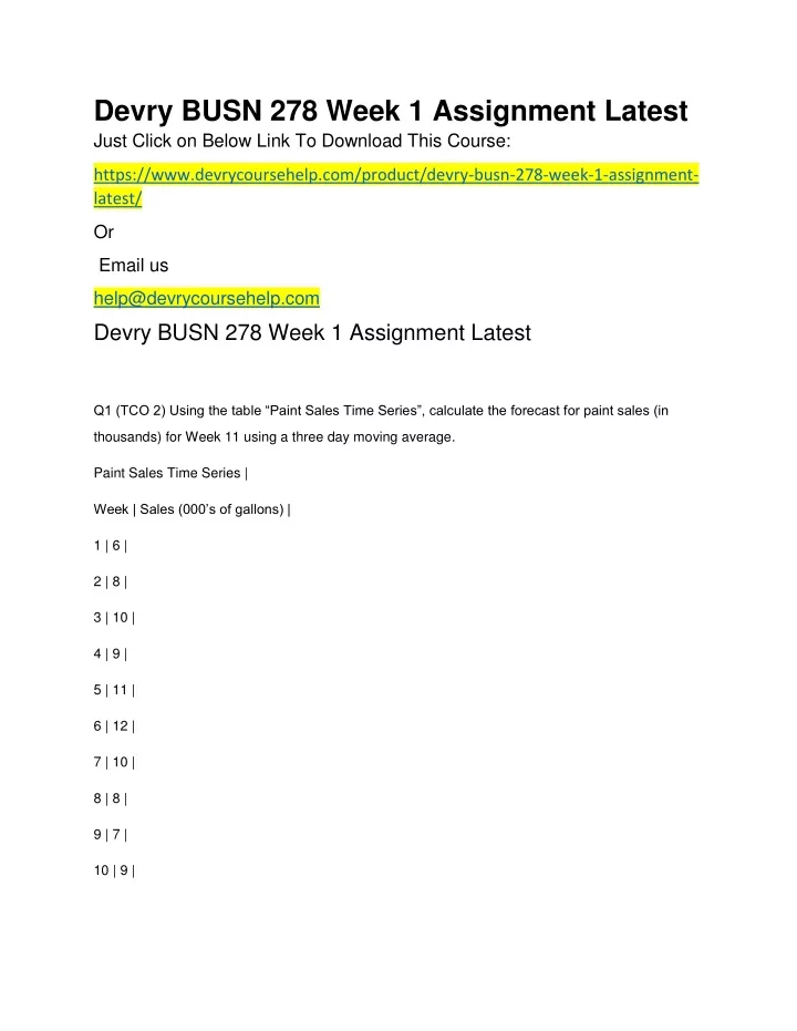
Devry BUSN 278 Week 1 Assignment Latest Just Click on Below Link To Download This Course: https://www.devrycoursehelp.com/product/devry-busn-278-week-1-assignment- latest/ Or Email us help@devrycoursehelp.com Devry BUSN 278 Week 1 Assignment Latest Q1 (TCO 2) Using the table “Paint Sales Time Series”, calculate the forecast for paint sales (in thousands) for Week 11 using a three day moving average. Paint Sales Time Series | Week | Sales (000’s of gallons) | 1 | 6 | 2 | 8 | 3 | 10 | 4 | 9 | 5 | 11 | 6 | 12 | 7 | 10 | 8 | 8 | 9 | 7 | 10 | 9 |
(TCO 2) Using the table “Paint Sales Time Series”, calculate the mean absolute deviation for a three day moving average. Paint Sales Time Series | Week | Sales (000’s of gallons) | 1 | 6 | 2 | 8 | 3 | 10 | 4 | 9 | 5 | 11 | 6 | 12 | 7 | 10 | 8 | 8 | 9 | 7 | 10 | 9 | Question : | (TCO 2) Using the table “Gasoline Sales Time Series”, calculate the forecast for gasoline sales (in thousands) for Week 13 using a three day weighted moving average. Use a weight of .60 for the most recent observation, .30 for the second most recent, and .10 for the third most recent. Gasoline Sales Time Series | Week | Sales (000’s of gallons) | 1 | 17 | 2 | 21 | 3 | 19 | 4 | 23 |
5 | 18 | 6 | 16 | 7 | 20 | 8 | 18 | 9 | 22 | 10 | 20 | 11 | 15 | 12 | 22 | 5. 5.| Question : | (TCO 2) Using the table “Gasoline Sales Time Series”, calculate the forecast for gasoline sales (in thousands) for Week 13 using exponential smoothing and a smoothing constant of .10. Gasoline Sales Time Series | Week | Sales (000’s of gallons) | 1 | 17 | 2 | 21 | 3 | 19 | 4 | 23 | 5 | 18 | 6 | 16 | 7 | 20 | 8 | 18 | 9 | 22 | 10 | 20 |
1. 1.| Question : | (TCO 3) Using the following information regarding actual sales for Seafood City, calculate the regression (trend) line: Sales for Seafood City ($) | Day | Week 1 | Week 2 | Monday | 1,700 | 1,800 | Tuesday | 1,900 | 2,000 | Wednesday | 2,100 | 2,100 | Thursday | 2,300 | 2,200 | Friday | 4,200 | 4,300 | Saturday | 4,400 | 4,600 | Sunday | 2,100 | 2,200 | 2. 2.| Question : | (TCO 3) Using the following information regarding actual sales for Sam’s Ski Supplies, project sales for March of Year 3 using simple linear regression: Sales for Sam’s Ski Supplies ($000s) | Month| First Year | Second Year | January | 380 | 400 | February | 340 | 360 | March | 320 | 330 | April | 280 | 290 | May | 265 | 270 | June | 230 | 235 | July | 220 | 230 | August| 200 | 205 | September | 210 | 220 |
October | 250 | 270 | November | 400 | 450 | December | 450 | 502 | | | 3. 3.| Question : | (TCO 3) Using the following information regarding actual sales for Sam’s Ski Supplies, calculate the seasonal ratio for January of Year 3: Sales for Sam’s Ski Supplies ($000s) | Month| First Year | Second Year | January | 380 | 400 | February | 340 | 360 | March | 320 | 330 | April | 280 | 290 | May | 265 | 270 | June | 230 | 235 | July | 220 | 230 | August| 200 | 205 | September | 210 | 220 | October | 250 | 270 | November | 400 | 450 | December | 450 | 502 | | 4. 4.| Question : | (TCO 3) Using the following information regarding actual sales for Paradise Pools, calculate the seasonal forecast of sales for April of Year 3:
Sales for Paradise Pools ($000s) | Month| First Year | Second Year | January | 84 | 84 | February | 80 | 82 | March | 88 | 98 | April | 100 | 120 | May | 150 | 160 | June | 200 | 210 | July | 240 | 250 | August| 220 | 215 | September | 180 | 195 | October | 160 | 165 | November | 120 | 130 | December | 92 | 100 | Download File Now