Download
1 / 31
310 likes | 330 Views
This article discusses the application of amplitude gains to seismic reflection data for better visualization of reflections and depths. It also explores common shot seismic profiles, migration techniques, trace interpolation, and imaging using earthquake waves.

E N D
The Amplitude Gain of Wiggles and Pixels for Reflection and Transmission Seismics By Robert Nowack Purdue University
Reflection Seismology In reflection seismology, seismic waves from surface sources are reflected from subsurface geologic structure.
This illustrates seismic waves propagating in the Earth from a surface source and reflected from subsurface geology (from Ikelle and Amundsen, 2005)
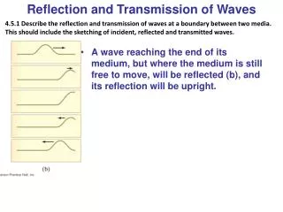
Common Shot Seismic Profile The first thing to note is that time is plotted vertically with the positive direction down. This is because for near vertically propagating waves which are reflected from subsurface structure, time can be used as a proxy for depth. The waves of interest are the reflected waves from interfaces in the Earth and these are hyperbolic in shape. All other waves including first arrivals are filtered out. From Liner (2005)
Amplitude gains are often applied to seismic reflection data to better see reflections at greater times and corresponding depths. a) Shows the original reflection data, b) shows seismic data that have been increased in amplitude by multiplying the traces by t compensating approximately for geometric spreading 1/R c) shows traces that are multipled by t**2 which then compensates also for some attenuation loss. d) shows a more complicated gain function applied. These gain functions can be removed if needed. Using automatic gain corrections or AGC, the amplitudes are increased over sliding windows down the data. Depending on the length of the window, different looks of the seismograms can result. However, AGC corrections can’t be removed.
In addition to gaining the data, muting out unwanted phases, as well as removing the source pulse through a proces called deconvolution is applied. With multiple shots and receivers along the surface, common offset profiles, or effective zero offset profiles, can be constructed.
The process of transforming seismic reflection data to an image of the geology is called seismic migration. For time migration the vertical axis is left in time and for depth migration the vertical axis is converted from time to depth.
The top plot is 11 km of effective zero offset reflection data across the Japan Trench. The bottom shows the result from time migration processing (from Claerbout, 1985)
Migrated seismic reflection data can be plotted in many different ways to highlight different features in the data. The recent book by Chopra and Marfurt (2007) describes a whole range of seismic attributes derived from the raw seismic data which can be used to best show different aspects of the data for interpretation.
Trace Interpolation For irregularly or sparsely spaced seismic traces, autoregressive trace interpolation can be used to densify or uniformize the station spacing of seismic data. This example shows an example of an interpolation for three linear waves recorded on sparse traces. Trace interpolation is now frequently used in the oil industry (e.g. Abma and Kabir, 2005) and more recently for teleseismic wavefield interpolation (e.g. Wilson and Guitton, 2007).
Visualization tools are now regularly used for the interpretation of processed reflection seismic data
3D Data Volume Top View(Kingdom Suite Software/Stratton Data)
Imaging using Earthquake Waves Imaging with seismic waves from distant earthquakes uses incident waves arriving from below and scattered by the local Earth structure beneath a seismic array.
For imaging using earthquake waves, the source time function of the earthquake source must either be removed or accounted for in the imaging. Traditional approaches have constructed so-called receiver functions in which the vertical component is assumed to be the signal from the earthquake source and is removed from the horizontal components by a process called deconvolution. New approaches attempt to deconvolve all the components of the seismic data. Alternatively, interferometric approaches are being developed that image the seismic data without first removing the earthquake source signal.
Synthetic test model from the 1993 Cascadia Experiment An idealized collisional zone model from Shragge et al. (2001). From this model, synthetics are computed for a teleseismic P-wave incident at the base of the model at 20 degrees.
Synthetic seismic data for the collisional zone model The synthetic scattered seismic data are for a P-wave at 20 degrees from the vertical incident from below the structure.
Gaussian beam migration imaging of synthetic data from the collisional zone model using the PpPp phase reflected from the free surface and the converted Ps Phase
The left plot shows a Gaussian beam migration image from a single earthquake source for the PpPs surface reflected phase showing the subduction zone structure in Oregon beneath the Pacific Northwest down to 100 km. The right plot is a ray-Born imaging result for the same event from Rondenay, et al. (2001).
Project Hi-CLIMB (Himalayan-Tibetan Continental Lithosphere During Mountain Building) • Over 210 broadband seismic station sites in central Tibet. • Deployed Between 2002 to 2005. • The linear component in Tibet (used in this study) is located over both the Lhasa and Qiangtangterranes. • Station spacing is around 3 to 10 km.
This shows a seismic image using Gaussian beam migration for crustal and very upper mantle structure in central Tibet (Nowack et al., 2010). The results from using wide-angle waves from SsPmP arrivals (red dots) are also shown (from Tseng, et al., 2009).
Wide-angle seismic body waves can also be transformed and processed to form a wavefield showing the velocity model. The left plot shows a wide-angle synthetic wavefield reduced in time with upper mantle triplication from the 410 and 660 km discontinuities. The right plot shows a transformed and processed wavefield reconstructing the original velocity model (from Nowack online seismology lecture notes, web.ics.purdue.edu/~nowack).
This illustrates the use of interferometry to convert global seismic data into effective reflection imaging (from Wapaneer, 2004) Travel-time tomography Green’s function retrieval Interferometric reflection imaging
References Abma, R. and N. Kabir (2005) Comparisons of interpolation methods, The Leading Edge, 24, 984-989. Chopra, S. and K. Marfurt (2007) Seismic Attributes for Prospect Identification and Reservoir Characterization, SEG, Tulsa. Claerbout, J.F. (1985) Imaging the Earth’s Interior, Blackwell. Kingdom Suite seismic visualization software (2011) Seismic Micro-Technology Inc., Houston TX. Ikelle, L.T. and L. Amundsen (2005) Introduction to Petroleum Seismology, SEG, Tulsa. Liner, C.L. (2007) Elements of 3D seismology, Pennwell, Tulsa. Nowack, R.L., W.P. Chen and T.L. Tseng (2010) Application of Gaussian beam migration to multi-scale imaging of the lithosphere beneath the Hi-CLIMB array in Tibet, Bull. Seism. Soc. Am., 100, 1743-1754. Rondenay, S., M.G. Bostock and J. Shragge (2001) Multiparameter two-dimensional inversion of scattered teleseismic body waves, 3, Applications to the Cascadia 1993 data set, J. Geophys. Res., 106, 30,795-30,808. Ruigrok, E., D. Draganov, and K. Wapenaar (2008) Global-scale seismic interferometry: theory and numerical examples, Geophys. Prosp., 56, 395-417.
References cont. Shragge, J., M.G. Bostock and S. Rondenay (2001) Multiparameter two-dimensional inversion of scattered teleseismic body waves, 2, Numerical examples, J. Geophys. Res. 106, 30,783-30,794. Stockwell, J. (2011) Geophysical image processing with Seismic Unix: GPGN 461/561 Lab, Center for Wave Phenomena, Colorado School of Mines. Stockwell, J. and J.K. Cohen (2007) The New SU User’s manual, Center for Wave Phenomena, Colorado School of Mines. Tseng, T.L., W.P. Chen, and R.L. Nowack (2009) Northward thinning of Tibetan crust revealed by virtual seismic profiles, Geophys. Res. Lett., 36, doi:10.1029/2009GL038252. Wapenaar, K. and D. Draganov (2004) Retrieving the Green’s function by cross-correlation: a comparison of approaches, Am. Geophys. Un. Fall Ann. Meeting, San Francisco. Wilson, C. and A. Guitton (2007) Teleseismic wavefield interpolation and signal extraction using high-resolution linear Radon transforms, Geohys. J. Int., 168, 171-181.