Chapter 2 Solutions of Equations in One Variable

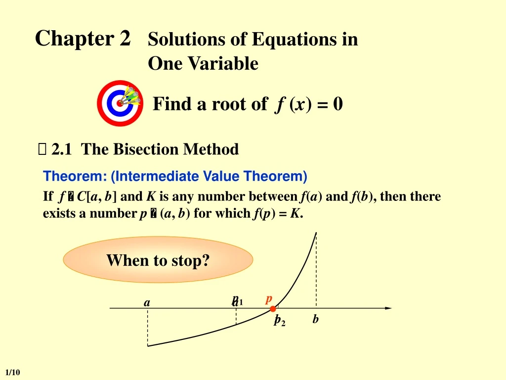
1. Find a root off (x) = 0 a b Chapter 2Solutions of Equations in One Variable  2.1 The Bisection Method Theorem: (Intermediate Value Theorem) If f C[a, b] and K is any number between f(a) and f(b), then there exists a number p  (a, b) for which f(p) = K. When to stop? p1 p a b p2 1/10

2. Chapter 2Solutions of Equations in One Variable -- The Bisection Method    p pN Theorem: Suppose that f C[a, b] and f(a) · f(b) < 0. The Bisection method generates a sequence { pn} (n = 0, 1, 2, …) approximating a zero p of f with when n  1. There exist sequences { pN } that diverge while | pN – pN – 1 | <   Proof: p.52 2/10

3. Chapter 2Solutions of Equations in One Variable -- The Bisection Method Algorithm: Bisection To find a solution to f (x) = 0 given the continuous function f on the interval [ a, b ], where f (a) and f (b) have opposite signs. Input: endpoints a, b; tolerance TOL; maximum number of iterations Nmax. Output: approximate solution p or message of failure. Step 1 Set i = 1; FA = f (a) ; Step 2 While ( i  Nmax) do steps 3-6 Step 3 Set p = a + ( b – a ) / 2 ; /* compute pi */ FP = f (p) ; Step 4 If ( FP == 0 ) or ( b  a ) / 2 < TOL then Output (p); STOP; /* successful */ Step 5 Set i ++; Step 6 If sign(FA) · sign(FP) > 0 then set a = p ; FA = FP ; Else set b = p ; /* update ai, bi */ Step 7 Output (Method failed after Nmax iterations); /* unsuccessful */ STOP. Why not p = ( a + b ) / 2 ? Why not FA· FP > 0? 3/10

4. Chapter 2Solutions of Equations in One Variable -- The Bisection Method ① Simple, only requires a continuous f ; ② Always converges to a solution. ① Slow to converge, and a good intermediate approximation can be inadvertently discarded; ② Cannot find multiple roots and complex roots. Note: Practically, we can sketch a graph of f(x) before applying the bisection method. Or use a subroutine to partition the interval into several sub-intervals [ak, bk] so that f (ak)·f (bk) < 0 even when f (a)·f (b) > 0. HW: p.54 #13, 15 4/10

5. Chapter 2Solutions of Equations in One Variable -- Fixed-Point Iteration equivalent Start from an initial approximation p0 and generate the sequence by letting pn = g( pn – 1 ), for each n 1. If the sequence converges to p and g is continuous, then Idea  2.2 Fixed-Point Iteration f (x) = 0 x = g (x) Fixed-point of g (x) Root of f (x) So basically we are done! I can’t believe it’s so simple! What’s the problem? Oh yeah? Who tells you that the method is convergent? 5/10

6. Chapter 2Solutions of Equations in One Variable -- Fixed-Point Iteration t0 t1 y=g(x) t0 y y y y y = x y = x y = x y = x y=g(x) t1 p0 p1 p p p0 p p1 y=g(x) y=g(x) x x x x t0 t0 t1 t1 p1 p0 p0 p p1     6/10

7. Chapter 2Solutions of Equations in One Variable -- Fixed-Point Iteration (1 – g’()) (p – q) = 0 Theorem: (Fixed-Point Theorem) Let g C[a, b] be such that g(x)  [a, b], for all x in [a, b]. Suppose, in addition, that g’ exists on (a, b) and that a constant 0 < k < 1 exists with |g’(x)|  k for all x  (a, b). Then, for any number p0 in [a, b], the sequence defined by pn = g( pn – 1 ), n 1, converges to the unique fixed point p in [a, b].    a. Let f(x) = g(x) – x. Proof: The Intermediate Value Theorem implies that f has a root, and hence ghas a fixed point. b. Prove by contradiction: Suppose p and q are both fixed points of g in [a, b] and p  q. The Mean Value Theorem implies that a number  exists between p and q with g(p) – g(q) = g’() (p – q). = p = q Contradiction! Hence the fixed point is unique. 7/10

8. Chapter 2Solutions of Equations in One Variable -- Fixed-Point Iteration c. g(x)  [a, b], for all x in [a, b] 0 Corollary: If gsatisfies the hypotheses of the Fixed-Point Theorem, then bounds for the error involved in using pn to approximate p are given by (for all n 1) and Proof (continued): pn is defined for all n 0 Proof: Can be used to control the accuracy The the value of k, the faster the convergence. smaller 8/10

9. Chapter 2Solutions of Equations in One Variable -- Fixed-Point Iteration Algorithm: Fixed-Point Iteration Find a solution to p = g(p) given an initial approximation p0. Input: initial approximation p0; tolerance TOL; maximum number of iterations Nmax. Output: approximate solution p or message of failure. Step 1 Set i = 1; Step 2 While ( i  Nmax) do steps 3-6 Step 3 Set p = g(p0); /* compute pi */ Step 4 If | p  p0 | < TOL then Output (p); /* successful */ STOP; Step 5 Set i ++; Step 6 Set p0 = p ; /* update p0 */ Step 7 Output (The method failed after Nmax iterations); /* unsuccessful */ STOP. 9/10

10. Chapter 2Solutions of Equations in One Variable -- Fixed-Point Iteration Example: Find the unique root of the equation x3 + 4x2 – 10 = 0 in [1, 2]. Using the following equivalent fixed-point forms with p0 = 1.5, which one is the best? (The root is approximately 1.365230013.)      But why? OK in [1, 1.5]. k 0.66  k 0.15 HW: p.64 #3, p.65 #19 10/10