Download
1 / 41
410 likes | 443 Views
Del Siegle explains the factors limiting a Pearson's correlation coefficient, such as homogeneous groups, unreliable measurements, nonlinear relationships, and clustered scores. He uses student examples to highlight how correlations can change with data addition.

E N D
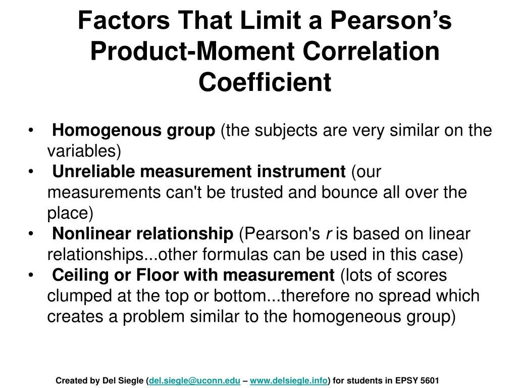
Factors That Limit a Pearson’s Product-Moment Correlation Coefficient • Homogenous group (the subjects are very similar on the variables) • Unreliable measurement instrument (our measurements can't be trusted and bounce all over the place) • Nonlinear relationship (Pearson's r is based on linear relationships...other formulas can be used in this case) • Ceiling or Floor with measurement (lots of scores clumped at the top or bottom...therefore no spread which creates a problem similar to the homogeneous group) Created by Del Siegle (del.siegle@uconn.edu – www.delsiegle.info) for students in EPSY 5601
Factors That Limit a Pearson’s Product-Moment Correlation Coefficient • Homogenous group (the subjects are very similar on the variables) • Unreliable measurement instrument (our measurements can't be trusted and bounce all over the place) • Nonlinear relationship (Pearson's r is based on linear relationships...other formulas can be used in this case) • Ceiling or Floor with measurement (lots of scores clumped at the top or bottom...therefore no spread which creates a problem similar to the homogeneous group) Created by Del Siegle (del.siegle@uconn.edu – www.delsiegle.info) for students in EPSY 5601
Imagine that we created a scatterplot of first graders’ weight and height. Notice how the correlation is around r=.60. . . . . . . . . . . . . . . . . . . . Height . Weight
Now let’s add data from second graders (assuming second graders are generally heavier and taller than first graders but the relationship between their weight and height is similar to first graders). Imagine that we created a scatterplot of first graders’ weight and height. Notice how the correlation is around r=.60. . . . . . . . . . . . . . . . . . . . . . . . . . . . . . . . . . . . . . . Height . Weight
We now have added third graders. Notice how the total scatterplot for first through third graders resembles r=.80 while each grade resembled r=.60. Now let’s add data from second graders (assuming second graders are generally heavier and taller than first graders but the relationship between their weight and height is similar to first graders). Imagine that we created a scatterplot of first graders’ weight and height. Notice how the correlation is around r=.60. . . . . . . . . . . . . . . . . . . . . . . . . . . . . . . . . . . . . . . . . . . . . . . . . . . . . . . . . . Height . Weight
Extending the scatterplot to fourth graders increases the value of r even more. Now let’s add data from second graders (assuming second graders are generally heavier and taller than first graders but the relationship between their weight and height is similar to first graders). We now have added third graders. Notice how the total scatterplot for first through third graders resembles r=.80 while each grade resembled r=.60. Imagine that we created a scatterplot of first graders’ weight and height. Notice how the correlation is around r=.60. . . . . . . . . . . . . . . . . . . . . . . . . . . . . . . . . . . . . . . . . . . . . . . . . . . . . . . . . . . . . . . . . . . . . . . . . . . . . Height . Weight
Now let’s add data from second graders (assuming second graders are generally heavier and taller than first graders but the relationship between their weight and height is similar to first graders). Imagine that we created a scatterplot of first graders’ weight and height. Notice how the correlation is around r=.60. Extending the scatterplot to fourth graders increases the value of r even more. We now have added third graders. Notice how the total scatterplot for first through third graders resembles r=.80 while each grade resembled r=.60. As we add fifth graders, we can see that the correlation coefficient is approaching r=.95 for first through fifth graders. . . . . . . . . . . . . . . . . . . . . . . . . . . . . . . . . . . . . . . . . . . . . . . . . . . . . . . . . . . . . . . . . . . . . . . . . . . . . . . . . . . . . . . . . . . . . . . . Height . Weight
Now let’s add data from second graders (assuming second graders are generally heavier and taller than first graders but the relationship between their weight and height is similar to first graders). Imagine that we created a scatterplot of first graders’ weight and height. Notice how the correlation is around r=.60. Extending the scatterplot to fourth graders increases the value of r even more. We now have added third graders. Notice how the total scatterplot for first through third graders resembles r=.80 while each grade resembled r=.60. The purpose of this demonstration is to illustrate that homogeneous groups . . . . . . . . . . . . . . . . . . . . . . . . . . . . . . . . . . . . . . . . . . . . . . . . . . . . . . . . . . . . . . . . . . . . . . . . . . . . . . . . . . . . . . . . . . . . . . . Height . Weight
Now let’s add data from second graders (assuming second graders are generally heavier and taller than first graders but the relationship between their weight and height is similar to first graders). Imagine that we created a scatterplot of first graders’ weight and height. Notice how the correlation is around r=.60. Extending the scatterplot to fourth graders increases the value of r even more. We now have added third graders. Notice how the total scatterplot for first through third graders resembles r=.80 while each grade resembled r=.60. The purpose of this demonstration is to illustrate that homogeneous groups produce smaller correlations than heterogeneous groups. . . . . . . . . . . . . . . . . . . . . . . . . . . . . . . . . . . . . . . . . . . . . . . . . . . . . . . . . . . . . . . . . . . . . . . . . . . . . . . . . . . . . . . . . . . . . . . . Height . Weight
Factors That Limit a Pearson’s Product-Moment Correlation Coefficient • Homogenous group (the subjects are very similar on the variables) • Unreliable measurement instrument (our measurements can't be trusted and bounce all over the place) • Nonlinear relationship (Pearson's r is based on linear relationships...other formulas can be used in this case) • Ceiling or Floor with measurement (lots of scores clumped at the top or bottom...therefore no spread which creates a problem similar to the homogeneous group) Created by Del Siegle (del.siegle@uconn.edu – www.delsiegle.info) for students in EPSY 5601
. . . . . . . . . . . . . . . . . . . . . . . . . . . . . . . . . . . . . . . . . . . . . . . . . . . . . . . Assume that the relationship between Variable 1 and Variable 2 is r = - 0.90. Variable 2 . Variable 1
If the instrument to measure Variable 1 were unreliable, the values for Variable 1 could randomly be smaller or larger. Variable 2 . . . . . . . . . . . . . . . . . . . . . . . . . . . . . . . . . . . . . . . . . . . . . . . . . . . . . . . . Variable 1
This would occur for all of the scores. Variable 2 . . . . . . . . . . . . . . . . . . . . . . . . . . . . . . . . . . . . . . . . . . . . . . . . . . . . . . . . Variable 1
Unreliable instruments limit our ability to see relationships. Variable 2 . . . . . . . . . . . . . . . . . . . . . . . . . . . . . . . . . . . . . . . . . . . . . . . . . . . . . . . . Variable 1
Factors That Limit a Pearson’s Product-Moment Correlation Coefficient • Homogenous group (the subjects are very similar on the variables) • Unreliable measurement instrument (our measurements can't be trusted and bounce all over the place) • Nonlinear relationship (Pearson's r is based on linear relationships...other formulas can be used in this case) • Ceiling or Floor with measurement (lots of scores clumped at the top or bottom...therefore no spread which creates a problem similar to the homogeneous group) Created by Del Siegle (del.siegle@uconn.edu – www.delsiegle.info) for students in EPSY 5601
. . . . . . . . . . . . . . . . . . . . . . . . . . . . . . . . . . . . . . . . . . . . . . . . . . . . . . . Imagine that each year couples were married they became slightly less happy. Happiness . Years’ Married
. . . . . . . . . . . . . . . . . . . . . . . . . . . . . . . . . . . . . . . . . . . . . . . . . . . . . . . . . . . . . . . . . . . . . . . . . . . . . . . . . . . . . . . . . . . . . . . . . . . . . . . . . . . . . . Imagine that after they are married for 7 years, they slowly become more happy each year. Happiness . Years’ Married
. . . . . . . . . . . . . . . . . . . . . . . . . . . . . . . . . . . . . . . . . . . . . . . . . . . . . . . . . . . . . . . . . . . . . . . . . . . . . . . . . . . . . . . . . . . . . . . . . . . . . . . . . . . . . . The negative correlation for the first 7 years… Happiness . Years’ Married
. . . . . . . . . . . . . . . . . . . . . . . . . . . . . . . . . . . . . . . . . . . . . . . . . . . . . . . . . . . . . . . . . . . . . . . . . . . . . . . . . . . . . . . . . . . . . . . . . . . . . . . . . . . . . . …cancels the positive relationship for the next 7 years. Happiness . Years’ Married
. . . . . . . . . . . . . . . . . . . . . . . . . . . . . . . . . . . . . . . . . . . . . . . . . . . . . . . . . . . . . . . . . . . . . . . . . . . . . . . . . . . . . . . . . . . . . . . . . . . . . . . . . . . . . . Pearson’s r would show no relationship (r=0.00) between year’s married and happiness even though the scatterplot clearly shows a relationship. Happiness . Years’ Married
. . . . . . . . . . . . . . . . . . . . . . . . . . . . . . . . . . . . . . . . . . . . . . . . . . . . . . . . . . . . . . . . . . . . . . . . . . . . . . . . . . . . . . . . . . . . . . . . . . . . . . . . . . . . . . This is an example of a curvilinear relationship. Pearson’s r is not an appropriate statistic for curvilinear relationships. Happiness . Years’ Married
. . . . . . . . . . . . . . . . . . . . . . . . . . . . . . . . . . . . . . . . . . . . . . . . . . . . . . . One of the assumptions for using Pearson’s r is that the relationship is linear. That is why the first step in correlation data analysis is to create a scatterplot. Happiness . Years’ Married
Factors That Limit a Pearson’s Product-Moment Correlation Coefficient • Homogenous group (the subjects are very similar on the variables) • Unreliable measurement instrument (our measurements can't be trusted and bounce all over the place) • Nonlinear relationship (Pearson's r is based on linear relationships...other formulas can be used in this case) • Ceiling or Floor with measurement (lots of scores clumped at the top or bottom...therefore no spread which creates a problem similar to the homogeneous group) Created by Del Siegle (del.siegle@uconn.edu – www.delsiegle.info) for students in EPSY 5601
. . . . . . . . . . . . . . . . . . . . . . . . . . . . . . . . . . . . . . . . . . . . . . . . . . . . . . . . . . . . . . . . . . . . . . . . . . . . . . . . . . . . . . . . Imagine that we are plotting the relationship between Variable 1 and Variable 2. . . . . . . . Variable 2 1 2 3 4 5 6 7 8 9 . 1 2 3 4 5 6 7 8 9 10 11 12 13 14 15 16 Variable 1
. . . . . . . . . . . . . . . . . . . . . . . . . . . . . . . . . . . . . . . . . . . . . . . . . . . . . . . . . . . . . . . . . . . . . . . . . . . . . . . . . . . . . . . . As values on Variable 1 increase, values on Variable 2 also increase. . . . . . . . Variable 2 1 2 3 4 5 6 7 8 9 . 1 2 3 4 5 6 7 8 9 10 11 12 13 14 15 16 Variable 1
. . . . . . . . . . . . . . . . . . . . . . . . . . . . . . . . . . . . . . . . . . . . . . . . . . . . . . . . . . . . . . . . . . . . . . . . . . . . . . . . . . . . . . . . As values on Variable 1 increase, values on Variable 2 also increase. . . . . . . . Variable 2 1 2 3 4 5 6 7 8 9 . 1 2 3 4 5 6 7 8 9 10 11 12 13 14 15 16 Variable 1
. . . . . . . . . . . . . . . . . . . . . . . . . . . . . . . . . . . . . . . . . . . . . . . . . . . . . . . . . . . . . . . . . . . . . . . . . . . . . . . . . . . . . . . . As values on Variable 1 increase, values on Variable 2 also increase. . . . . . . . Variable 2 1 2 3 4 5 6 7 8 9 . 1 2 3 4 5 6 7 8 9 10 11 12 13 14 15 16 Variable 1
. . . . . . . . . . . . . . . . . . . . . . . . . . . . . . . . . . . . . . . . . . . . . . . . . . . . . . . . . . . . . . . . . . . . . . . . . . . . . . . . . . . . . . . . As values on Variable 1 increase, values on Variable 2 also increase. . . . . . . . Variable 2 1 2 3 4 5 6 7 8 9 . 1 2 3 4 5 6 7 8 9 10 11 12 13 14 15 16 Variable 1
. . . . . . . . . . . . . . . . . . . . . . . . . . . . . . . . . . . . . . . . . . . . . . . . . . . . . . . . . . . . . . . . . . . . . . . . . . . . . . . . . . . . . . . . As values on Variable 1 increase, values on Variable 2 also increase. . . . . . . . Variable 2 1 2 3 4 5 6 7 8 9 . 1 2 3 4 5 6 7 8 9 10 11 12 13 14 15 16 Variable 1
. . . . . . . . . . . . . . . . . . . . . . . . . . . . . . . . . . . . . . . . . . . . . . . . . . . . . . . . . . . . . . . . . . . . . . . . . . . . . . . . . . . . . . . . . . . . . . . Variable 2 1 2 3 4 5 6 7 8 9 . 1 2 3 4 5 6 7 8 9 10 11 12 13 14 15 16 Variable 1
. . . . . . . . . . . . . . . . . . . . . . . . . . . . . . . . . . . . . . . . . . . . . . . . . . . . . . . . . . . . . . . . . . . . . . . . . . . . . . . . . . . . . . . . Suppose that the top score on the instrument used to measure Variable 2 is 9 (in other words there is a “ceiling” on Variable 2’s measurement instrument). . . . . . . . Variable 2 1 2 3 4 5 6 7 8 9 . 1 2 3 4 5 6 7 8 9 10 11 12 13 14 15 16 Variable 1
. . . . . . . . . . . . . . . . . . . . . . . . . . . . . . . . . . . . . . . . . . . . . . . . . . . . . . . . . . . . . . . . . . . . . . . . . . . . . . . . . . . . . . . . Our subjects can continue to have higher scores on Variable 1, but they are restricted on Variable 2. . . . . . . . Variable 2 1 2 3 4 5 6 7 8 9 . 1 2 3 4 5 6 7 8 9 10 11 12 13 14 15 16 Variable 1
. . . . . . . . . . . . . . . . . . . . . . . . . . . . . . . . . . . . . . . . . . . . . . . . . . . . . . . . . . . . . . . . . . . . . . . . . . . . . . . . . . . . . . . . Our subjects can continue to have higher scores on Variable 1, but they are restricted on Variable 2. . . . . . . . Variable 2 1 2 3 4 5 6 7 8 9 . 1 2 3 4 5 6 7 8 9 10 11 12 13 14 15 16 Variable 1
. . . . . . . . . . . . . . . . . . . . . . . . . . . . . . . . . . . . . . . . . . . . . . . . . . . . . . . . . . . . . . . . . . . . . . . . . . . . . . . . . . . . . . . . Our subjects can continue to have higher scores on Variable 1, but they are restricted on Variable 2. . . . . . . . Variable 2 1 2 3 4 5 6 7 8 9 . 1 2 3 4 5 6 7 8 9 10 11 12 13 14 15 16 Variable 1
. . . . . . . . . . . . . . . . . . . . . . . . . . . . . . . . . . . . . . . . . . . . . . . . . . . . . . . . . . . . . . . . . . . . . . . . . . . . . . . . . . . . . . . . Our subjects can continue to have higher scores on Variable 1, but they are restricted on Variable 2. . . . . . . . Variable 2 1 2 3 4 5 6 7 8 9 . 1 2 3 4 5 6 7 8 9 10 11 12 13 14 15 16 Variable 1
. . . . . . . . . . . . . . . . . . . . . . . . . . . . . . . . . . . . . . . . . . . . . . . . . . . . . . . . . . . . . . . . . . . . . . . . . . . . . . . . . . . . . . . . Our subjects can continue to have higher scores on Variable 1, but they are restricted on Variable 2. . . . . . . . Variable 2 1 2 3 4 5 6 7 8 9 . 1 2 3 4 5 6 7 8 9 10 11 12 13 14 15 16 Variable 1
. . . . . . . . . . . . . . . . . . . . . . . . . . . . . . . . . . . . . . . . . . . . . . . . . . . . . . . . . . . . . . . . . . . . . . . . . . . . . . . . . . . . . . . . . . . . . . . Variable 2 1 2 3 4 5 6 7 8 9 . 1 2 3 4 5 6 7 8 9 10 11 12 13 14 15 16 Variable 1
. . . . . . . . . . . . . . . . . . . . . . . . . . . . . . . . . . . . . . . . . . . . . . . . . . . . . . . . . . . . . . . . . . . . . . . . . . . . . . . . . . . . . . . . We can see that the ceiling on Variable 2 is causing us to have a lower correlation than if our subjects were able to continue to score higher on Variable 2. . . . . . . . Variable 2 1 2 3 4 5 6 7 8 9 . 1 2 3 4 5 6 7 8 9 10 11 12 13 14 15 16 Variable 1
. . . . . . . . . . . . . . . . . . . . . . . . . . . . . . . . . . . . . . . . . . . . . . . . . . . . . . . . . . . . . . . . . . . . . . . . . . . . . . . . . . . . . . . . Our subjects can continue to have higher scores on Variable 1, but they are restricted on Variable 2. . . . . . . . Variable 2 1 2 3 4 5 6 7 8 9 . 1 2 3 4 5 6 7 8 9 10 11 12 13 14 15 16 Variable 1
. . . . . . . . . . . . . . . . . . . . . . . . . . . . . . . . . . . . . . . . . . . . . . . . . . . . . . . . . . . . . . . . . . . . . . . . . . . . . . . . . . . . . . . . When a variable is measured with an instrument that has a ceilings (or floor), we obtain a lower correlation coefficients than if the variable were measured with an instrument that did not have a ceiling (or floor). . . . . . . . Variable 2 1 2 3 4 5 6 7 8 9 10 . 1 2 3 4 5 6 7 8 9 10 11 12 13 14 15 16 Variable 1
Factors That Limit a Pearson’s Product-Moment Correlation Coefficient • Homogenous group (the subjects are very similar on the variables) • Unreliable measurement instrument (our measurements can't be trusted and bounce all over the place) • Nonlinear relationship (Pearson's r is based on linear relationships...other formulas can be used in this case) • Ceiling or Floor with measurement (lots of scores clumped at the top or bottom...therefore no spread which creates a problem similar to the homogeneous group) Created by Del Siegle (del.siegle@uconn.edu – www.delsiegle.info) for students in EPSY 5601