Download
1 / 59
590 likes | 604 Views
Explore the use of optimal control to enhance accuracy and reduce numerical dissipation in solving Euler equations. Learn about the theory, results, and applications of this innovative approach.

E N D
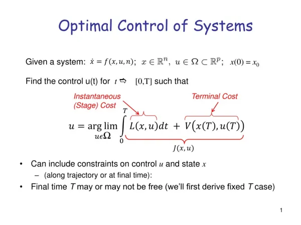
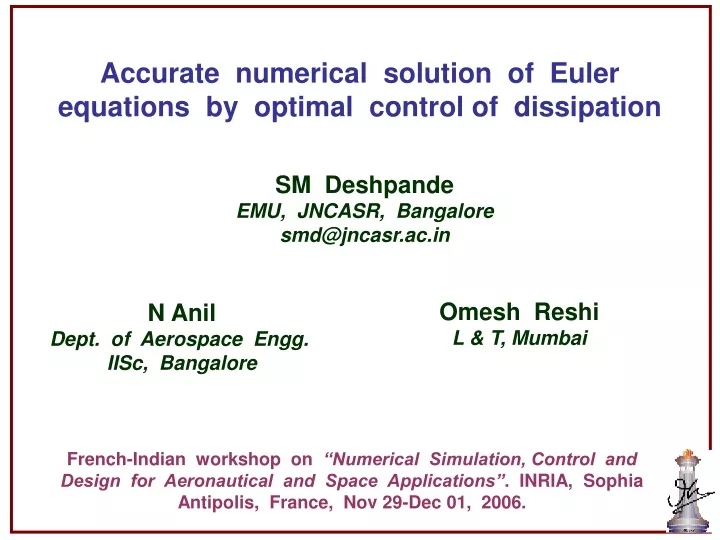
Accurate numerical solution of Euler equations by optimal control of dissipation SM Deshpande EMU, JNCASR, Bangalore smd@jncasr.ac.in Omesh Reshi L & T, Mumbai N Anil Dept. of Aerospace Engg. IISc, Bangalore French-Indian workshop on “Numerical Simulation, Control and Design for Aeronautical and Space Applications”. INRIA, Sophia Antipolis, France, Nov 29-Dec 01, 2006.
OUTLINE • Introduction to KFVS • Basic theory of m-KFVS • Numerical Results • Optimal control of dissipation • A numerical test case • Conclusions
INTRODUCTION TO KFVS Consider the 1D Euler equations which are moments of the 1D Boltzmann equation in the Euler limit where F - Maxwellian velocity distribution function
INTRODUCTION TO KFVS The Euler equations can be written as is the moment function vector The inner product is defined as
INTRODUCTION TO KFVS Using CIR splitting, 1D Boltzmann equation gives Taking moments, we get KFVS Euler equations The split fluxes are given by
INTRODUCTION TO KFVS Consider the CIR split Boltzmann equation Using suitable finite difference approximations The mpde analysis gives KFVS – first order accurate and dissipative !
INTRODUCTION TO KFVS • Numerical dissipation can be reduced by using • higher order upwind schemes • In the case of 1D, second order scheme requires • 5 points in the stencil • Is it possible to develop a scheme which requires • only 3 point stencil but still gives results better • than first order and close to second order ?
BASIC THEORY OF MKFVS MCIR Splitting The modified CIR splitting is defined as The mpde based on MCIR splitting is given by
BASIC THEORY OF MKFVS … Taking moments we get mpde at Euler level The modified split fluxes are given by • By tuning we can control dissipation and • order of accuracy
BASIC THEORY OF MKFVS … Mathematical models for : Consider the mpde When
BASIC THEORY OF MKFVS … = Numerical kinematic viscosity When • Particles with contribute maximum to • Particles with contribute very little to
BASIC THEORY OF MKFVS … The choice • Low velocity particles for which - Contribute very little to • High velocity particles for which - Contribute max. to
BASIC THEORY OF MKFVS … Another choice • Low velocity particles for which - Contribute max. to • High velocity particles for which - Contribute very little to
BASIC THEORY OF MKFVS … Consider the steady 1D Boltzmann equation with a BGK model for the collision term Using the the solution is given by Assuming to be constant over
BASIC THEORY OF MKFVS … • The low velocity molecules are almost always lost • While high velocity molecules are lost negligibly, • i.e., they travel over without any collision • The choice is consistent with the earlier argument • but doesn’t have closed form expressions for the split fluxes • The second choice leads to much simpler formulae • for split fluxes
BASIC THEORY OF MKFVS … For the modified split fluxes are given by • - full flux, - kfvs fluxes, non - dimensional parameter • mkfvs fluxes are simpler and similar to kfvs fluxes • Takes almost the same amount of time as kfvs fluxes • Smooth for all Mach number range • Continuous and differentible functions
BASIC THEORY OF MKFVS … Dissipation Analysis : The mpde for 1D Euler equations based on mkfvs is given by The dissipation matrix is given by
BASIC THEORY OF MKFVS … Dissipation Analysis : The numerical kinematic viscosity is given by • Here are the eigenvalues of the matrix D • For large values of the eigenvalues
BASIC THEORY OF MKFVS … Max of the matrix D for increase in
NUMERICAL RESULTS 1D inviscid test cases: • Convergent Divergent nozzle problem • Shock tube problem 2D inviscid test cases: • Subsonic flow past Williams airfoil • Transonic flow past NACA 0012 airfoil • Supersonic flow past NACA 0012 airfoil
NUMERICAL RESULTS … Convergent – divergent nozzle
NUMERICAL RESULTS … Convergent – divergent nozzle test case: • Governing equations are quasi-one-dimensional • Steady flow • Number of grid points : 60 • Computations are performed with
NUMERICAL RESULTS … Non-dimensional pressure along the nozzle using Non-dimensional value along the nozzle using
NUMERICAL RESULTS … Variation of density along the shock tube. No. of points = 500
NUMERICAL RESULTS … Non-dimensional value along the shock tube
NUMERICAL RESULTS … Variation of density for higher values of
NUMERICAL RESULTS … Role of in numerical simulations: • Increase of enhances accuracy • has been used to suppress wiggles
NUMERICAL RESULTS … Features of 2D cell centred FVM solver based on m-KFVS • m-KFVS fluxes for flux evaluation • modified kinetic wall and outer boundary conditions • Local time stepping • LUSGS for convergence acceleration
NUMERICAL RESULTS … Subsonic flow past Williams airfoil M = 0.15 aoa = 0.0 Grid points = 50000
NUMERICAL RESULTS … m-KFVS KFVS Entropy contours of m-KFVS method are compared with KFVS and q-KFVS q-KFVS
NUMERICAL RESULTS … KFVS m-KFVS Pressure contours of m-KFVS method are compared with KFVS and q-KFVS q-KFVS
NUMERICAL RESULTS … Cp – distribution: kfvs, m-kfvs and exact Flap Main airfoil
NUMERICAL RESULTS … Transonic flow past NACA 0012 airfoil M = 0.85 aoa = 1.0 320x120 structured grid
NUMERICAL RESULTS … KFVS m-KFVS Pressure contours of m-KFVS method are compared with KFVS and q-KFVS q-KFVS
NUMERICAL RESULTS … Cp-Plot of m-KFVS are compared with KFVS and q-KFVS
NUMERICAL RESULTS … Pressure distribution on unstructured grid Cp-Plot of m-KFVS are compared with KFVS and q-KFVS
NUMERICAL RESULTS … Supersonic flow past NACA 0012 airfoil M = 1.2, aoa = 0.0 320x120 structured grid
NUMERICAL RESULTS … m-KFVS KFVS Pressure contours of m-KFVS method are compared with KFVS and q-KFVS q-KFVS
NUMERICAL RESULTS … Comments on m-KFVS: • It gives results as accurate as second • order accurate q-KFVS • It does not have spurious wiggles near • shock, which are present in q-KFVS
OPTIMAL CONTROL OF DISSIPATION • Consider the 2D subsonic flow past NACA 0012 airfoil • Accurate capture of suction peak depends on numerical • entropy generated by the scheme • The low dissipative m-KFVS method captures the suction • peak more accurately compared to KFVS • Further, by optimal control of dissipation parameter , • we can get even better accuracy Optimisation Problem : Cost function = Sum of squares of entropy at cells
OPTIMAL CONTROL OF DISSIPATION Discrete adjoint approach Minimise: The cost function I The discrete form of the cost function is given by where - Vector of conserved variables - Dissipation control variables vector - Number of cells in the computational domain
OPTIMAL CONTROL OF DISSIPATION Subject to:The governing state equations Where are the fluxes along coordinate directions Few observations: • The cost function doesn’t explicitly depend on • It depends on through its dependence on solution • The number of design variables = N = Number of cells
OPTIMAL CONTROL OF DISSIPATION The first variation in the cost function is given by The first variation in the state equation is given by
OPTIMAL CONTROL OF DISSIPATION At any cell i the first variation is given by The above equation can be written in expanded notation
OPTIMAL CONTROL OF DISSIPATION Introducing the vector of adjoint variables, and using the state equation as a constraint Collecting all the terms which are coefficients of and equating them to zero we get the adjoint euqtion for cell i where is the adjoint residual for the cell
OPTIMAL CONTROL OF DISSIPATION Further expanding Introducing a pseudo time stepping We have used TAPENADE to compute the gradients
OPTIMAL CONTROL OF DISSIPATION The adjoint variables are then substituted in the equation for cost function variation Again TAPENADE is used to compute the gradient
OPTIMAL CONTROL OF DISSIPATION One of the early and simplest methods is steepest descent method in which Using the above method the cost function will decrease Now better methods are available. We have here used the above steepest descent method as a first step The values of can be updated using
A NUMERICAL TEST CASE Comments on the m-KFVS-AD solver • Non-linear m-KFVS solver written in C++ • m-KFVS-AD solver written in FORTRAN 77 • TAPENADE is used to get the subroutines, • which are used to compute the gradients • in the AD solver
A NUMERICAL TEST CASE Subsonic flow past NACA 0012 Airfoil • M = 0.63, aoa = 2.0o • Unstructured grid with 4733 points • Non-linear solver – 2D cell centred FVM • based on m-KFVS