Download
1 / 14
140 likes | 244 Views
Chapter 17.5. Poisson ANCOVA. Classic Poisson Example. N umber of deaths by horse kick, for each of 16 corps in the Prussian army, from 1875 to 1894 The risk of death did not change over time in Guard Corps. Is there a similar lack of trend in the 1 st ,2 nd , and 3 rd units ?.

E N D
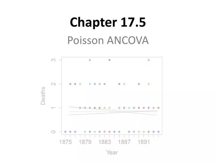
Chapter 17.5 Poisson ANCOVA
Classic Poisson Example • Number of deaths by horse kick, for each of 16 corps in the Prussian army, from 1875 to 1894 • The risk of death did not change over time in Guard Corps. • Is there a similar lack of trend in the 1st,2nd, and 3rd units ?
2. Execute analysis & 3. Evaluate model glm1 <- glm(deaths~year*corps, family = poisson(link=log), data=horsekick)
2. Execute analysis & 3. Evaluate model glm1 <- glm(deaths~year*corps, family = poisson(link=log), data=horsekick)
2. Execute analysis & 3. Evaluate model • glm1 <- glm(deaths~year*corps, family = • poisson(link=log), data=horsekick) • deviance(glm1)/df.residual(glm1) • [1] 1.134671 • Dispersion parameter assumed to be 1 • As a general rule, dispersion parameters approaching 2 (or 0.5) indicate possible violations of this assumption
Side note: Over-dispersion > deviance(glm2)/df.residual(glm2) [1] 4.632645
State population and whether sample is representative. • Decide on mode of inference. Is hypothesis testing appropriate? • State HA / Ho pair, tolerance for Type I error Statistic: Non-PearsonianChisquare(G-statistic) Distribution: Chisquare
7. ANODEV. Calculate change in fit (ΔG) due to explanatory variables. > library(car) > Anova(glm1, type=3) Analysis of Deviance Table (Type III tests) Response: deaths LR ChisqDfPr(>Chisq) year 0.61137 1 0.4343 corps 1.27787 3 0.7344 year:corps 1.27073 3 0.7361
7. ANODEV. Calculate change in fit (ΔG) due to explanatory variables. > Anova(glm1, type=3) … LR ChisqDfPr(>Chisq) year 0.61137 1 0.4343 corps 1.27787 3 0.7344 year:corps 1.27073 3 0.7361 > anova(glm1, test="LR") … Terms added sequentially (first to last) Df Deviance Resid. DfResid. DevPr(>Chi) NULL 79 95.766 year 1 0.00215 78 95.764 0.9630 corps 3 1.14678 75 94.617 0.7658 year:corps 3 1.27073 72 93.347 0.7361
Assess table in view of evaluation of residuals. • Residuals acceptable • Assess table in view of evaluation of residuals. • Reject HA: The four corps show the same lack of trend in deaths by horsekick over two decades (ΔG=1.27, p=0.736) • Analysis of parameters of biological interest. • βyear was not significant – report mean deaths/unit-yr • (56 deaths / 20 years) / 4 units = 0.7 deaths/unit-year
library(pscl) library(Hmisc) library(car) corp.id <- c("G","I","II","III") horsekick <- subset(prussian, corp %in% corp.id) names(horsekick) <- c("deaths","year","corps") glm0 <- glm(deaths ~ 1, family = poisson(link = log), data = horsekick) # intercept only glm1 <- glm(deaths ~ year*corps, family = poisson(link = log), data = horsekick) plot(fitted(glm1),residuals(glm1),pch=16, xlab="Fitted values", ylab="Residuals") plot(residuals(glm1), Lag(residuals(glm1)), xlab="Residuals", ylab="Lagged residuals", pch=16) sum(residuals(glm1, type="pearson")^2)/df.residual(glm1) deviance(glm1)/df.residual(glm1) plot(horsekick$year,horsekick$deaths, pch=16, axes=F, xlab="Year", col=horsekick$corps, ylab="Deaths") axis(1, at=75:94, labels=1875:1894) axis(2, at=0:4) box() Anova(glm1, type=3, test.statistic="LR") anova(glm1, test="LR") species <- read.delim("http://www.bio.ic.ac.uk/research/mjcraw/therbook/data/species.txt") plot(Species~Biomass, data=species, pch=16) lm1 <- lm(Species~Biomass, data=species) plot(fitted(lm1),residuals(lm1), pch=16, xlab="Fitted values", ylab="Residuals", main="GLM") glm2<-glm(Species~Biomass, data=species, family=poisson) plot(fitted(glm2),residuals(glm2), pch=16, xlab="Fitted values", ylab="Residuals", main="GzLM") deviance(glm2)/df.residual(glm2)