Download
1 / 66
660 likes | 916 Views
Static Equilibrium Asset Pricing. Chapter 3. Capital Asset Pricing Model (CAPM). Section 3.1. CAPM. Original portfolio-based asset pricing model Most all modern asset pricing builds from this Sharpe/Lintner (and sort of Treynor) 1960’s Assumptions All investors price takers

E N D
Static Equilibrium Asset Pricing Chapter 3
Capital Asset Pricing Model (CAPM) Section 3.1
CAPM • Original portfolio-based asset pricing model • Most all modern asset pricing builds from this • Sharpe/Lintner (and sort of Treynor) 1960’s • Assumptions • All investors price takers • Common information/beliefs • Portfolios evaluated on means and variances • Pick some mean/variance efficient portfolio • Equilibrium • Market portfolio = tangent portfolio • Market portfolio is mean/var efficient • At market price (return) equilibrium, no way to better mean/var asset portfolio
Portfolio change experiment (should look familiar from micro)
Guts of CAPM • This isn’t very testable • Assume market portfolio is MV efficient
Black CAPM (borrowing constraints) Section 3.1.2
Risk free rates • Assume lending, but no borrowing • This can get much more complex in terms of rates • We are just glancing at this quickly • People vary in their risk preferences (risky portfolios now differ) • Assume all portfolios on frontier • All portfolios are weighted sums of two fixed mutual funds (separation) • This implies that the market portfolio is also a weighted sum of these and lies on the frontier itself • Can yield a CAPM, but risk free replaced with “zero beta” portfolio • The key idea here is that the existence of a risk free asset is not critical to a CAPM like beta pricing relationship
CAPM Applications in real portfolios Section 3.1.3
Last figures • These last two figures are important in relation to the CAPM • The CAPM makes no statement about where individual returns sit relative to their standard deviation (Sharpe ratios) • The Sharpe ratio does define the slope of the line through the tangent (and often market) portfolio • The CAPM does make a strong statement about the slope of the line in the second figure (The Security Market line) • Expected returns of all portfolios should lie on this line • Some tests of the CAPM statistically test the “distance” of returns from the SML • Active manager strive to achieve “alpha” which puts them above this line
Investment management • The CAPM also says a lot of about performance and investment management • Investors should not “pay for beta risk” • If an investment manager delivers a higher expected return, but is still on the SML (zero alpha), investors could just do this themselves by borrowing (leverage) and buying more of the market • This does also correspond to moving out beyond the tangent portfolio in the std/return plots too • Why pay someone for something you can do yourself • This intuition will carry over into our logic for arbitrage pricing
A simple picture of return/beta from Malkiel and Fama/French
Black/Litterman CAPM (casual description) • Standard portfolio selection generates “crazy” portfolio weights • Noise in expected returns creates big swings in weights • Black/Litterman • Set a kind of prior for returns that follow a standard CAPM • W considers how strong beliefs are in current sample estimates versus CAPM prior • Fed into standard portfolio optimization • Black/Litterman sort of casual (see book) • This is a form of empirical Bayes estimation
Multifactor models/Arbitrage Pricing Section 3.2.1
Thoughts on arbitrage • Key concept in finance • Portfolios that generate same payoffs should have same price • Very powerful • Does not rely on preferences • Can sometimes be limited in scope • Examples • Arbitrage Pricing Theory (APT) • Black/Scholes • Much of fixed income pricing
Arbitrage pricing • Important model • And modeling style (arbitrage) • Few assumptions about preferences • Related to other models such as Black/Scholes • Also, related to CAPM, and modern multi-factor (Fama/French) factor models
Excess return and zero cost strategies • We often state stuff in terms of excess returns • They have many convenient features • One is that investors can add any excess return to a portfolio with no concern for budgets • They are “zero cost” investments • Increase risky asset, borrow risk free
Basic arbitrage • Buy portfolio • Then short (allowed) units of the market portfolio • This will give you a completely risk free payout • Absence of arbitrage implies these free lunches do not exist • Therefore, • What about for individual securities?
Individual securities • This does not say that each alpha is zero • This depends on thinking about N big, and lots of securities • If there are groups where alpha is big then • Buy them • Neutralize market risk • Take arbitrage profits • Alpha for individuals must stay close to zero
Technical aside • Does this imply: • No, this is only a limiting result • Some of these expected returns might be nonzero, but they generally need to be “pretty small” • This can get technical fast • See Campbell (pp 56-57) for proof that APT implies that: • Proof is not super difficult, but will skip
What else can screw up for APT? • Factor structure not correct • Other factors • Idiosyncratic errors not independent • This is a problem • You need to be able to build the diversified factor portfolios that let you ignore idiosyncratic risk • This is related to the “other factors” issue
Multifactor models Section 3.2.2
Implications • Linear pricing (expected returns) structure (like CAPM) • MV efficient set is spanned by K factor portfolios • Why? • Think about portfolio on frontier with some idiosyncratic risk • One could replicate this exactly in terms of expected returns and systematic risk (factor risk) by purchasing factor portfolios • This would have same expected return and smaller variance • So no portfolio exists on the frontier that we can’t do better using pure factor returns • Practical aside: • Some factor portfolios can be directly purchased as exchange traded funds (ETF’s)
Empirical history of APT • Principle components • Macro factors • Portfolio factors • This has been the most successful
Conditional CAPM and factors Section 3.2.3
Conditional CAPM and multifactors • A conditional CAPM can be mapped into a multifactor model • Allow beta to move around through time • This is now a two factor model • Factor 2 is the market return “scaled” by info variable z(t) • This is a kind of synthetic strategy which increases/decreases market holdings depending on z(t)
Empirical evidence (light) Section 3.3.1 Test methodology
CAPM: Three basic tests • Time series • Cross sectional • Fama/MacBeth
Time series approach • Could run for one security, and test alpha=0 • Joint tests for alpha(i)=0 • Assume errors iid • Asymptotic Chi-squared test on weighted squared alpha (3.45) • Adjusts for beta uncertainty in model • Finite sample F-test (3.46) • Distance of market Sharpe ratio from tangency Sharpe ratio
Cross-sectional approach • Estimate beta’s from time series regressions • Then run cross-section regression (no intercept) • This is again a chi-squared test • Estimation needs GLS (a’s not independent/cross sectional dependence) • Asymptotic test statistic (3.51)
Fama-MacBeth(1973) • Cross-section with time series changes • Useful test • Used outside of finance too (rolling cross sectional) • Method: • Run time series regression to get Beta’s • Then cross-sectional regression at each time t • FM get standard errors • Problem: Does not adjust for beta estimation • Interesting: Can be done with changing beta’s
Rolling Fama/MacBeth • Set window (1,T) • Estimate beta in window • Estimate CAPM in T+1 • Set window (2,T+1) • Estimate beta in window • Estimate CAPM T+2
Returns and characteristics • Cross sectional F/M useful for adding other things to CAPM testing • In true CAPM world other stuff should not matter • Many flavors of this • X can be any firm level characteristic (profits, growth, size) • Drop beta • More factors • Trading strategy interpretation (see 3.55)
Choosing test assets • Occasionally individual stocks are grouped into portfolios for testing • All asset pricing theory should hold for portfolios • For example “high beta” and “low beta” portfolios replace R(it) • Designed to get more power/precision in tests • Can be controversial (see references on p66)
Empirical features Section 3.3.2
Individual asset return time series features • Nearly uncorrelated • Prices near random walk • Non normal distributions at frequencies less than quarterly • Persistent volatility • Increasing when prices fall (Leverage effect) • Most of academic research is on cross-sectional features • This is where AP models operate
CAPM • Early tests in 1970’s • Works but, • Beta small • Barely significant • Working less well after 1960 • Remember Malkiel picture
Size • Size = market capitalization (shares*price) • Smaller firms have higher returns • Often in the month of January • The “January effect” • See next figure • Note: portfolio sort technology
Value • Extremely old strategy (Graham, Dodd, Cottle(1934), Buffet) • Key ratio (something)/(market cap) • Something = book value, dividends, earnings • High ratio • Cheap stocks • Buy!!
Momentum • Persistence in returns • Autocorrelations are a little more subtle than zero • Negative at highest (intraday/daily) frequencies • Positive at mid range (monthly-yearly) • Strategy: Buy recent winners • Negative (reversals) at long horizons (5 years) • Strategy: Buy losers
Modern research midrange • Formation period • Previous 6-12 months • Sort (maybe 5-10 portfolios) based on returns in this period • Wait 1 month • Strategy test in next month after this • Long winner portfolio, short loser • Several different flavors of this • All strategies together (next figure) • MOM • SMB (small minus big, size) • HML (book/market, value) • Much of this data is available at Ken French’s website