Download
1 / 21
250 likes | 528 Views
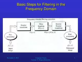
Digital Image Processing Lecture 9: Filtering in Frequency Domain. Prof. Charlene Tsai. 2-D Discrete. For an MxN matrix All 1-D properties transfer into 2-D Some more properties useful for image processing. Separability.

E N D
Digital Image Processing Lecture 9: Filtering in Frequency Domain Prof. Charlene Tsai
2-D Discrete • For an MxN matrix • All 1-D properties transfer into 2-D • Some more properties useful for image processing.
Separability • The 1st term depends only on x and u, and the 2nd term depends on y and v. • Advantage: computing DFT of all the columns first, then computing the DFT of all the rows of the result. 1st term 2nd term
(con’d) • 1D Fourier pair: (a) Original image (b) DFT of each row of (a), using x & u (c) DFT of each column of (b), using y & v
Convolution Theory • Review: • How to convolve an image M with a spatial filter S in spatial domain? • If Z,X,Y are the DFT’s of z=x*y, x and y respectively, then Z=X.Y (convolution theory) • We can perform the same operation (convolution) in frequency domain • Pad S with 0, so same size as M; denote the new matrix S’ • Perform DFT on M and S’ to obtain F(M) and F(S’) • Perform inverse DFT on F(M).F(S’) to get F-1 • M*S is F-1 • Great saving for a large filter. elt-by-elt product
Shifting • Review: In 1-D, if multiplying each element xn of vector x by (-1)n we swap the left and right halves of the Fourier transform. • In 2-D, the same principle applies if multiplying all elements xm,n by (-1)m+n before the transform. A B D C C D B A An FFT After shifting
Filtering • Our basic model for filtering in the frequency domain is • We’ll briefly discuss 3 types of filters in the order of increasing smoothness: • Ideal • Butterworth • Gaussian • Preprocessing: F is shifted so that the DC coefficient is in the center. filter Fourier transform of image to be smoothed result
Ideal Filtering:Low-Pass (ILPF) • The low-frequency components are toward the center. • Multiplying the transform by a matrix to remove or minimize the values away from the center. • Ideal low-pass matrix H • The inverse DFT of H.F is the smoothed image. D(u,v) is distance from the origin of the Fourier transform, shifted to the center
Demo An image with its Fourier spectrum. The superimposed circles have radii of 5, 15, 30, 80, and 230
Results D=5 D=30 D=15 D=80 D=230
Ideal Filtering:High-Pass (IHPF) • Opposite to low-pass filtering: eliminating center and keeping the others. D0=15 D0=30 D0=80
Butterworth Filtering: Low-Pass (BLPF) • Unlike ILPF, BLPF does not have a clear cutoff between passed and filtered frequencies. n is the order of the filter
Demo • n=2 and D0 equal the 5 radii D0=5 D0=15 D0=30 D0=80 D0=230
Butterworth Filtering: High-Pass (BHPF) D0=15 D0=30 D0=80
Gaussian Filtering: Low-Pass (GLPF) • We mentioned Gaussian once in the section for spatial filtering. • Will discuss more in detail in image restoration. • Gaussian filter in frequency domain: • The inverse is also a Gaussian. • We may replace by D0, which is the cutoff frequency.
Demo D0=5 D0=15 D0=30 D0=80 D0=230
Gaussian Filtering: High-Pass (GHPF) D0=15 D0=30 D0=80
In-class Exercise • Q. What is the Fourier transform of the average filtering using the 4 immediate neighbors of point (x,y), but excluding itself?
Summary • To perform filtering in frequency domain, do the following steps: • The Fourier transform of the image is shifted, so that the DC coefficient is in the center. (multiply the image by (-1)x+y) • Create the filter • Multiply it by the image transform • Invert the result • Multiplying the result by (-1)x+y. • The relationship between the corresponding high- and low-pass filters: