Download

1 / 37
380 likes | 398 Views
Learn about kinematic GPS in real-time and post-processing, ambiguity resolution techniques, and challenges in achieving precise positioning. Explore RTK and multiple baseline solutions.

E N D
Part IV KINEMATIC GPS AND AMBIGUITY RESOLUTION PROBLEM GS609 This file can be found on the course web page: http://geodesy.eng.ohio-state.edu/course/gs609/ Where also GPS reference links are provided
Kinematic GPS Positioning • What is kinematic GPS? • In kinematic mode the so-called rover receiver is moving with respect to the base, or maybe multiple rover receivers are moving with respect to each other and a base (or multiple base) station • Kinematic positioning is usually associated with real-time operation, however, the data collected in kinematic mode can be processed in the post-mission mode for higher accuracy • Thus, kinematic GPS positioning is performed either in real-time or post-processing
Kinematic GPS Positioning • Real-time kinematic GPS can be performed based on DGPS (WADGPS) services (thus, based on pseudoranging), as we discussed earlier, or • Can be done based on the user’s own base station, which usually supports precise, phase-based differential positioning • In real-time mode, the rover must communicate with the base via radio modem • In any case, the positioning can be done only after the integer ambiguities have been resolved • For very long baselines, kinematic positioning can be done based on real-valued ambiguities, if the integers cannot be resolved due to a high noise level • results in the loss of accuracy ( up to 10 cm per coordinate for baselines > 20 km, and more for baselines > 100 km)
Real-time Precise Kinematic GPS Positioning (RTK) • Requires real-time data transfer(radio link) – thus limited to shorter distanced, 10-20 km, depending on radio communication (limited reliability of data transfer) • Limited alsodue to the increasing atmospheric effects that prevent reliable ambiguity resolution (applies to any long-range GPS) • Requires use of carrier phase measurements(millimeter-level noise) • Exact determination of integer ambiguities is critical • In the static scenario, the changing satellite geometry allows for separation of the ambiguities from the constant station geometry • In the kinematic scenario ambiguity resolution is more difficult due to the motion of the station and the satellites (even more challenging for real-time)
Real-time Precise Kinematic GPS Positioning • Exact determination of integer ambiguities is critical(continued) • It must be done On-The-Fly (OTF) • It must be done fast • Presence of Anti Spoofing (AS) does not allow for instantaneous ambiguity resolution using four-measurement filter (i.e. two phase and two range observations) – longer and uninterrupted tracking is required to smooth the larger noise or some alternative techniques must be applied • Naturally SA (selective availability) does not make it easier either! • Luckily, SA was turned off in May 2000! However, AS remains the major problem, as pseudorange data have higher noise, as opposed to a no-AS case.
Epoch-by-epoch widelane ambiguity N1-N2 combination Under AS AS-free
Several Ambiguity resolution Techniques: • Ambiguity search (candidate solutions for four base satellite-other satellite pairs, centered about the real value solution, are chosen; the combination that gives the smallest root mean square error for the position is taken as the best solution) • Ambiguity function (uses no information from the range observations; the maximum for the ambiguity function determines the correct solution) • Ambiguity reparametrization (minimizes the correlation between the ambiguity integers and the elongation of the confidence ellipsoid; transformation is applied to the covariance matrix of DD integer estimates) • Kalman filtering (enables OTF over baselines of 100km or more; requires atmospheric modeling for longer baselines) • All methods come up with some real-valued ambiguity estimates first, and then apply some tricks to get them fixed to the right (hopefully) integers
Another Ambiguity Resolution method for Real-time Kinematic GPS • Multiple (or dual) baseline solution is an enhanced approach to ambiguity resolution for longer baselines (i.e., there are two or more base stations whose data can be used with the rover receiver data in any combination) • improves positioning performance by reducing the effects of GPS error spatial decorrelation • reduces the reference station noise • ultimately - enhances the performance of the OTF resolution, providing the closure check (N12=N1R-N2R) for the reference-rover ambiguities, that are resolved for each baseline On-The-Fly (subscripts 1 and 2 denote two base stations, R stands for roving receiver) • problem: limited capacity of data-link (doubled, or further multiplied for more than two base stations, amount of data) • Again, this method can be applied to post-processing of kinematic data, eliminating the communication problem
N 32.7km 30.2km 36.8km 31.6km
Mean and STD of the rover coordinates (differences from the known position)
Real-time Precise Kinematic GPS Positioning • Solution strategy/conditions: • Real-time ambiguity resolution • Minimum of four satellites must be tracked (after ambiguities are solved) • Least-squares batch solution • Kalman filtering • Uses data up to the epoch of observation • Processes data only once
Postprocessing of Kinematic GPS Data • Solution strategy/conditions: • Minimum of four satellites must be tracked (after ambiguities are solved) • Typically processes data twice • first run through the data determines integer ambiguities • second run estimates the rover positions • Can directly use the real-time algorithms • Least-squares batch solution • Kalman filtering/smoothing • uses data up to the epoch of observation (filtering) • uses the whole dataset (smoothing)
There are many ambiguity resolution techniques for a single baseline solution, one of them being ambiguity search based on four measurement filter, as presented below This method works well for shorter baselines, and under no AS (lower noise on pseudorange) it may become a simple, single epoch solution, where the real-valued ambiguities are just rounded to the nearest integers (but AS is in effect now, and is likely to remain so) So, let’s take a look at the ambiguity search technique
GPS Carrier Phase Ambiguity Fixing • four-measurement filter Phase observations can be expressed as linear combinations provides estimates for N1 and N2, as well as iono term and geometric distance combined with tropospheric effect
GPS Carrier Phase Ambiguity Fixing • Search technique • ambiguity search based on candidate solutions obtained from the four measurement filter • implementation of linear combinations of GPS phases: widelane and geometry-free combinations
GPS Carrier Phase Ambiguity Fixing • Search technique(cont.) • simultaneous estimation of widelane and geometry-free (double difference) ambiguities using combinations of four independent GPS code and phase observations (four-measurement filter) for four primary satellites (including the base satellite) • for short baselines (10-15km) differential ionospheric effects are constrained to zero, for longer baselines they are estimated • implementation of the least-squares ambiguity search, based on the estimated widelane (N1- N2 ) and geometry free (N1- 77/60 N2 ) ambiguities to resolve N1 and N2 for the primary satellites
GPS Carrier Phase Ambiguity Fixing • Search technique(cont.) • once ambiguities are resolvedfor the primary satellites, the rover position can be determined, and subsequently, the rest of the ambiguities can be resolved, and final rover positioning can be carried out • with the dual frequency GPS receivers and minimum of five satellites ambiguities are resolved within a few epochs of time • with only four satellites available, the lack of geometric strength might prevent from finding the correct solution
Integer Ambiguity Search Algorithm • Integer Search Algorithm • pick four primary satellites (highest elevation, best geometry) • the primary satellites are used to identify the potential solutions • the secondary group of satellites is needed to identify the correct solution among the potential solutions • evaluate geometry-free combination and determine double-differenced widelaneinteger candidates for the primary satellites (using four measurement filter)
Integer Ambiguity Search Algorithm • geometry-free condition • widelane • used in four measurement filter mode • unknowns: geometric range+troposphere, ionospheric effect, widelane and geometry-free ambiguities
Integer Ambiguity Search Algorithm • L1 and L2 phase ambiguity estimates • large abrupt changes in K1 and K2 indicate cycle slips on the primary satellites, and search is restarted
Integer Ambiguity Search Algorithm • establish the search window, based on the standard deviations of the widelane and geometry-free noise level, centered at the real-valued ambiguity estimates • determine all candidates N1and N2 within the search window • total number of combinations: k1*k2*k3, where k1, k2 and k3 are number of potential solutions (candidates of N1 and N2 pairs) for first, second and third pair of the primary satellites • define a set of positions in space for the rover receiver for every set of candidate integers • the sum of squares of residuals q of all the phase measurements over continuous epochs is used as a measure of the quality of a potential solution
Integer Ambiguity Search Algorithm v is a residual m is a number of continuous epochs n is number of satellites per epoch • ratio test - conducted between the smallest and the second smallest sum of squares q1 and q0 • if the ratio is larger than a certain criterion (here, 3), for at least 5 consecutive epochs, the position with the smallest sum of squared residuals is chosen as a correct solution • resolve ambiguities for the secondary satellites • rover positioning
Ambiguity Resolution read data satellites < 4 satellites >= 4 if first time or after restart: pick base and primary SVs continue from previous epoch: change in primary satellites ? restart restart Yes evaluate geom-free No can fix ambiguities cycle slip on prim. sat. cannot fix OK
Ambiguity Resolution ambiguities not fixed from previous epoch ambiguities fixed from previous epoch 4-meas filter to get NW check for cycle slips on the rest of satellites search window for NW and NGeom-free for primary satellites fix cycle slips and/or missing ambiguities N1 and N2 integer candidates
Ambiguity Resolution rover positioning for all candidate combinations fix ambs for the rest of SVs rover positioning sum of squared residuals for phase obs. for all candidate positions return to data read ambs. fixed for primary SVs ratio test failure 5-times success
Single frequency case • In case only L1 data are available, the above technique (or any other L1/L2 based method) cannot be used • Ambiguity is treated as another unknown and estimated in one common adjustment together with positions coordinates, clock parameters, etc., depending on the differential mode chosen – i.e., single or double differencing • All un-modeled error sources (such as ionosphere) affect all the estimates • Sequential adjustment with double differences is usually successful with single frequency data, i.e., if one ambiguity can be resolved and fixed to its integer value, the adjustment is repeated with one less unknown, to fix another ambiguity, etc. • Naturally, for longer baselines this might not work at all, as ionospheric effects will grow significantly.
Ambiguity Decorrelation: Concept • Double-differenced ambiguities are strongly correlated • Ambiguity decorrelation method removes or decreases correlation between double-difference ambiguities • As a consequence, the elongation of the ambiguity search space is significantly decreased assuring faster, more reliable search
Ambiguity Decorrelation: Procedure • Float Solution: • Integer Least-Squares Estimate • Decorrelation (transformation) of ambiguities • Actual integer ambiguity estimation (sequential conditional adjustment, search of the ambiguities, validation)
Ambiguity Decorrelation: Solution • Integer Least-Squares Estimate • target function: • has no standard solution (no ordinary least-squares problem). • The simplest solution: rounding to the nearest integer will give the correct answer only if the covariance matrix is diagonal, i.e., all the least-squares ambiguities are fully decorrelated
Ambiguity Decorrelation: Solution • Integer Least-Squares Estimate (cont.) • Thus, if decorrelated, the problem is reduced to minimizing independent squares: • Now rounding to the nearest integer can be applied
Ambiguity Decorrelation: Solution • Goal: replace the space of all integers Zm with smaller subset, based on the above target function, chosen as a region bounded by a hyper-ellipsoid • Result: ambiguity search space, centered at the real-valued solution; its shape depends on the covariance matrix (diagonalized), and size is controlled by the selected positive constant which is downscaled during the search • The integer solution is located inside this hyper-ellipsoid (one of the integer sets will minimize the target function)
Ambiguity Decorrelation: Solution • Search space for the two-dimensional case (two ambiguities): • Corresponding search bounds derived from the sum-of-squares structure
Ambiguity Decorrelation: Solution • Ambiguity transformation based on the conditional adjustment (sequential conditional least-squares ambiguities are fully decorrelated): • Transformed covariance and ambiguities: • Transformation is invertible, i.e.:
Ambiguity Decorrelation: Example • Input Data • dimension of the ambiguity vector • estimated vector of float ambiguities • their covariance matrix (lower triangular part) • Output • integer ambiguities • conditional variances • transformation matrix
Ambiguity Decorrelation: Example Input: -28490.856 65752.629 38830.366 5003.708 -29196.069 -297.658 -22201.028 51235.837 30257.780 3899.403 -22749.185 -159.278 Output: -28451 65749 38814 5025 -29165 -278 -22170 51233 30245 3916 -22725 -144