Download

1 / 39
390 likes | 544 Views
Computing Minimum-cardinality Diagnoses by Model Relaxation. Sajjad Siddiqi National University of Sciences and Technology (NUST) Islamabad, Pakistan. Consistency-based Diagnosis. NOT AND. C. Abnormal observation : A B D. A. X. D. Y. B. System model :

E N D
Computing Minimum-cardinality Diagnoses by Model Relaxation SajjadSiddiqi National University of Sciences and Technology (NUST) Islamabad, Pakistan
Consistency-based Diagnosis NOT AND C Abnormal observation : A B D A X D Y B System model : okX (A C) okY (B C) D Health variables: okX, okY Observables: A, B, D Nonobservable: C
Consistency-based Diagnosis C Abnormal observation : A B D A X D Y B System model : okX (A C) okY (B C) D Find values of (okX, okY) consistent with : (0, 0), (0, 1), (1, 0) OR {okX=0, okY=0}, …
Consistency-based Diagnosis System model over health variables(okX, okY, …) observables nonobservables Given observation , diagnosis is assignment to health variables consistent with Consider minimum-cardinality diagnoses Cardinality is the number of failing components in a diagnosis
Decomposable Negation Normal Form (DNNF) or • DAG of nested and/or • Conjuncts share no variable (decomposable) and Min-cardinality as well as min-cardinality diagnoses can be computed efficiently using DNNF or X3 and X1 X2
Compilation-based Approach System Model DNNF Compile Bottleneck Query Evaluator
Previous Method: Hierarchical Diagnosis Significantly reduces number of health variables – through Abstraction Requires only 160 health variables for c1908; c1908 has 880 gates Able to compile larger systems (Siddiqi and Huang, 2007)
Previous Method: Hierarchical Diagnosis Without Abstraction: Requires 6 healthvariables: okU, okV, okE, okB, okJ, okA
Previous Method: Hierarchical Diagnosis • Abstraction:{U,V,E,A} • Treats self contained sub-systems (E) as single components (cones): Requires 4 healthvariables: okU, okV, okE, okA
Previous Method: Hierarchical Diagnosis {E,A} is a an abstract min-cardinality diagnosis {E}, {J}, {B}are min-cardinality diagnoses of coneE. {J,A}, {B,A} are deduced as more min-cardinality diagnoses Need to find abnormal observation for coneE
Previous Method: Diagnosis of Cones Reorder{E,A} as {A,E} (deeper gates first) Propagate normal values in the circuit (input values in given observation) Propagate faults in the order they appear in diag. Sets the required abnormal obs for cone E
Previous Method Again Compilation becomes a bottleneck for very large systems – even after abstraction
New Method Combines abstraction, model relaxation (node splitting), and search to scale up Compiles the abstraction of a relaxed model instead of the original Applies two stage branch-and-bound search to compute minimum-cardinality diagnoses
Node Splitting Splits Y Y1’ and Y2’ are clones of Y (Choi et al., 2007)
Node Splitting Splits gate B
Node Splitting Some components may come out of cones The components in the abstraction of the split system form a superset of the set of components in the original abstraction The abstract min-cardinality diagnoses (once computed correctly) of the split system form a superset of the set of abstract min-cardinality diagnoses of the original
Search for minimum cardinality (First Stage) ∆ and ∆’ – models of original and split system e – a given assignment to variables in ∆ e – the compatible assignment to corresponding clones in the split system For example, if e = {B = b} then e = {B’ = b}
Search for minimum cardinality ∆’ provides basis for computing lower bounds on minimum cardinality for B-n-B search min_card(∆ | e) >= min_card(∆’ | ee) if e contains a complete assignment to split variables then min_card(∆ | e) == min_card(∆’ | ee)
Search for minimum cardinality B-n-B search in the space of assignments s to split variables S At each node compute min_card(∆’ | eess) At leaf nodes we get candidate minimum cardinalites Elsewhere, we get lower bounds to prune search
Search for minimum cardinality A good Seed for search In the given observation, if k components output values inconsistent with the normal values then k is the upper bound on the minimum cardinality.
Search for minimum cardinality Variable and value ordering Nogood-based scoring heuristic similar to (Siddiqi and Huang, 2009): Every value of a variable X is associated with a score S(X = x) Score of X, S(X), is the average of the scores of its values Vars and values with higher scores are preferred.
Search for minimum cardinality Variable and value ordering During search if X is assigned a value x then S(X = x) += new_bound – cur_bound cur_bound = bound before the assignment new_bound = bound after the assignment Early Backtracking
Search for diagnoses (Second Stage) First Strategy if e contains a complete assignment to split variables then min_card_diags(∆|e) == min_card_diags(∆’|ee) Search in the space of assignments to split variables; enumerate all min-card diagnoses at those leaf nodes where cardinality is minimum.
Search for Diagnoses Second Strategy Search in the space of assignments to health-vars Partial assignment to h-vars == partial diagnosis Enumerate all valid min-cardinality diagnoses.
Search for Diagnoses First Strategy Can efficiently compute very large number of diagnoses at leaf nodes by evaluating the DNNF Often resulted in very large search spaces even when the number of diagnoses was small Second Strategy Efficient only when the number of diagnoses was reasonably small
Combined Approach; benefit from both Systematic search in both spaces simultaneously: Search starts in the space of assignments to health variables At each search node, another search is performed in the space of assignments to split variables; IF REQUIRED.
Combined Approach Search on health variables Validate each partial diagnosish at each node If h is valid and card(h) < mincard, then continue search; else backtrack h is validiff: h is consistent with the model + observation h can be extended to a valid min-card diagnosis HOW???
Combined Approach Validate partial diagnosish: B-n-B Search for complete assignment to split varsS such that for each partial assignment s ∆’|heessis consistent AND card (h) + min_card(∆’|heess) <= mincard If such a complete assignment s exists then his valid; otherwise his invalid
Combined Approach Diagnoses At each node where h is valid compute min-card diagnoses as: {h}xmin_card_diags(∆’|heess) Union of all such diagnoses is the complete set of min-card diagnoses [redundancy is an issue]
Combined Approach <h1, s1, D1> okX = true okX = false <h2, s2, D2> <h3, s3, D3> h2 h1 h3 h1 min-card diagnoses = D1 D2 D3 (may overlap)
Avoiding Redundancy - 1 If s1 == s2 then D1 D2 <h1, s1, D1> okX = true okX = false <h2, s2, D2> <h3, s3, D3> h2 h1 h3 h1 Solution: At each node, keep passing `the assignment to split variables used’ to the children nodes, AND…
Avoiding Redundancy - 1 At each node with partial diagnosis h: Let sp = assignment to split vars used at the parent node First check if h is valid under sp: YES: Don’t search, don’t enum diagnoses NO: Search for a new assignment to split vars and enum diagnoses only if found
Avoiding Redundancy - 2 During search treat the all recorded diagnoses (so far) as nogoods Watch literals scheme (as in Satisfiability): As soon as all but one broken component in a recorded diagnosis have been assumed as broken, that remaining broken component is forced to be healthy
Combined Approach Variable and Value Ordering Same selection heuristic as in the first stage; scores try to minimize search on split vars Let search on split vars explored p nodes, when okX was assigned a value okx, then S(okX=okx) += 1/p If search is not performed at a node p = ½ of the value used at the parent
Combined Approach Variable and Value Ordering Initial scores: S(okX = true) = 0 S(okX = false) = failure probability of X (Siddiqi & Huang 11) Effectively orders components according to decreasing value of their failure probabilities
Diagnosis of Cones Same as in the previous method with some extra care: All clones must be assigned the same value during value and fault propagation When reordering components in abstract diagnosis, original depth values for components must be used despite changes due to splitting
Experiments Use ISCAS85 circuits Observations (inputs/outputs) randomly generated Multiple instances per circuit
Experiments New method solves most of the cases on every circuit (except c6288) Previous method cannot solve any case beyond c2670 New method is either as fast as the previous, or 4 times faster, or 2 orders of magnitude faster.
Summary New tool to compute minimum-cardinality diagnoses of a faulty system employing model relaxation, abstraction and search Solves non-trivial diagnostic cases on large systems, not possible before Significantly faster than the previous on cases solvable by both