Download
1 / 253
2.53k likes | 2.69k Views
Discrete and Categorical Data. William N. Evans Department of Economics/MPRC University of Maryland. Part I. Introduction. Introduction. Workhorse statistical model in social sciences is the multivariate regression model Ordinary least squares (OLS)

E N D
Discrete and Categorical Data William N. Evans Department of Economics/MPRC University of Maryland
Part I Introduction
Introduction • Workhorse statistical model in social sciences is the multivariate regression model • Ordinary least squares (OLS) • yi = β0 + x1iβ1+ x2iβ2+… xkiβk+ εi • yi = xi β + εi
Linear model yi = + xi + i • and are “population” values – represent the true relationship between x and y • Unfortunately – these values are unknown • The job of the researcher is to estimate these values • Notice that if we differentiate y with respect to x, we obtain • dy/dx =
represents how much y will change for a fixed change in x • Increase in income for more education • Change in crime or bankruptcy when slots are legalized • Increase in test score if you study more
Put some concretenesson the problem • State of Maryland budget problems • Drop in revenues • Expensive k-12 school spending initiatives • Short-term solution – raise tax on cigarettes by 34 cents/pack • Problem – a tax hike will reduce consumption of taxable product • Question for state – as taxes are raised, how much will cigarette consumption fall?
Simple model: yi = + xi + i • Suppose y is a state’s per capita consumption of cigarettes • x represents taxes on cigarettes • Question – how much will y fall if x is increased by 34 cents/pack? • Problem – many reasons why people smoke – cost is but one of them –
Data • (Y) State per capita cigarette consumption for the years 1980-1997 • (X) tax (State + Federal) in real cents per pack • “Scatter plot” of the data • Negative covariance between variables • When x>, more likely that y< • When x<, more likely that y> • Goal: pick values of and that “best fit” the data • Define best fit in a moment
Notation • True model • yi = + xi + i • We observe data points (yi,xi) • The parameters and are unknown • The actual error (i)is unknown • Estimated model • (a,b) are estimates for the parameters (,) • ei is an estimate of i where • ei=yi-a-bxi • How do you estimate a and b?
Objective: Minimize sum of squared errors • Min iei2 = i(yi – a – bxi)2 • Minimize sum of squared errors (SSE) • Treat (+) and (-) errors equally • Over or under predict by “5” is the same magnitude of error • “Quadratic form” • The optimal value for a and b are those that make the 1st derivative equal zero • Functions reach min or max values when derivatives are zero
The model has a lot of nice features • Statistical properties easy to establish • Optimal estimates easy to obtain • Parameter estimates are easy to interpret • Model maximizes prediction • If you minimize SSE you maximize R2 • The model does well as a first order approximation to lots of problems
Discrete and Qualitative Data • The OLS model work well when y is a continuous variable • Income, wages, test scores, weight, GDP • Does not has as many nice properties when y is not continuous • Example: doctor visits • Integer values • Low counts for most people • Mass of observations at zero
Downside of forcing non-standard outcomes into OLS world? • Can predict outside the allowable range • e.g., negative MD visits • Does not describe the data generating process well • e.g., mass of observations at zero • Violates many properties of OLS • e.g. heteroskedasticity
This talk • Look at situations when the data generating process does not lend itself well to OLS models • Mathematically describe the data generating process • Show how we use different optimization procedure to obtain estimates • Describe the statistical properties
Show how to interpret parameters • Illustrate how to estimate the models with popular program STATA
Types of data generating processes we will consider • Dichotomous events (yes or no) • 1=yes, 0=no • Graduate high school? work? Are obese? Smoke? • Ordinal data • Self reported health (fair, poor, good, excel) • Strongly disagree, disagree, agree, strongly agree
Count data • Doctor visits, lost workdays, fatality counts • Duration data • Time to failure, time to death, time to re-employment
Recommended Textbooks • Jeffrey Wooldridge, “Econometric analysis of cross sectional and panel data” • Lots of insight and mathematical/statistical detail • Very good examples • William Greene, “Econometric Analysis” • more topics • Somewhat dated examples
Course web page • www.bsos.umd.edu/econ/evans/jpsm.html • Contains • These notes • All STATA programs and data sets • A couple of “Introduction to STATA” handouts • Links to some useful web sites
STATA Resources Discrete Outcomes • “Regression Models for Categorical Dependent Variables Using STATA” • J. Scott Long and Jeremy Freese • Available for sale from STATA website for $52 (www.stata.com) • Post-estimation subroutines that translate results • Do not need to buy the book to use the subroutines
In STATA command line type • net search spost • Will give you a list of available programs to download • One is Spostado from http://www.indiana.edu/~jslsoc/stata • Click on the link and install the files
Part II A brief introduction to STATA
STATA • Very fast, convenient, well-documented, cheap and flexible statistical package • Excellent for cross-section/panel data projects, not as great for time series but getting better • Not as easy to manipulate large data sets from flat files as SAS • I usually clean data in SAS, estimate models in STATA
Key characteristic of STATA • All data must be loaded into RAM • Computations are very fast • But, size of the project is limited by available memory • Results can be generated two different ways • Command line • Write a program, (*.do) then submit from the command line
Sample program to get you started • cps87_or.do • Program gets you to the point where can • Load data into memory • Construct new variables • Get simple statistics • Run a basic regression • Store the results on a disk
Data (cps87_do.dta) • Random sample of data from 1987 Current Population Survey outgoing rotation group • Sample selection • Males • 21-64 • Working 30+hours/week • 19,906 observations
Major caveat • Hardest thing to learn/do: get data from some other source and get it into STATA data set • We skip over that part • All the data sets are loaded into a STATA data file that can be called by saying: use data file name
Housekeeping at the top of the program • * this line defines the semicolon as the ; • * end of line delimiter; • # delimit ; • * set memork for 10 meg; • set memory 10m; • * write results to a log file; • * the replace options writes over old; • * log files; • log using cps87_or.log,replace; • * open stata data set; • use c:\bill\stata\cps87_or; • * list variables and labels in data set; • desc;
------------------------------------------------------------------------------------------------------------------------------------------------------------ • > - • storage display value • variable name type format label variable label • ------------------------------------------------------------------------------ • > - • age float %9.0g age in years • race float %9.0g 1=white, non-hisp, 2=place, • n.h, 3=hisp • educ float %9.0g years of education • unionm float %9.0g 1=union member, 2=otherwise • smsa float %9.0g 1=live in 19 largest smsa, • 2=other smsa, 3=non smsa • region float %9.0g 1=east, 2=midwest, 3=south, • 4=west • earnwke float %9.0g usual weekly earnings • ------------------------------------------------------------------------------
Constructing new variables • Use ‘gen’ command for generate new variables • Syntax • gen new variable name=math statement • Easily construct new variables via • Algebraic operations • Math/trig functions (ln, exp, etc.) • Logical operators (when true, =1, when false, =0)
From program • * generate new variables; • * lines 1-2 illustrate basic math functoins; • * lines 3-4 line illustrate logical operators; • * line 5 illustrate the OR statement; • * line 6 illustrates the AND statement; • * after you construct new variables, compress the data again; • gen age2=age*age; • gen earnwkl=ln(earnwke); • gen union=unionm==1; • gen topcode=earnwke==999; • gen nonwhite=((race==2)|(race==3)); • gen big_ne=((region==1)&(smsa==1));
Getting basic statistics • desc -- describes variables in the data set • sum – gets summary statistics • tab – produces frequencies (tables) of discrete variables
From program • * get descriptive statistics; • sum; • * get detailed descriptics for continuous variables; • sum earnwke, detail; • * get frequencies of discrete variables; • tabulate unionm; • tabulate race; • * get two-way table of frequencies; • tabulate region smsa, row column cell;
Results from sum • Variable | Obs Mean Std. Dev. Min Max • -------------+-------------------------------------------------------- • age | 19906 37.96619 11.15348 21 64 • race | 19906 1.199136 .525493 1 3 • educ | 19906 13.16126 2.795234 0 18 • unionm | 19906 1.769065 .4214418 1 2 • smsa | 19906 1.908369 .7955814 1 3 • -------------+--------------------------------------------------------
Detailed summary • usual weekly earnings • ------------------------------------------------------------- • Percentiles Smallest • 1% 128 60 • 5% 178 60 • 10% 210 60 Obs 19906 • 25% 300 63 Sum of Wgt. 19906 • 50% 449 Mean 488.264 • Largest Std. Dev. 236.4713 • 75% 615 999 • 90% 865 999 Variance 55918.7 • 95% 999 999 Skewness .668646 • 99% 999 999 Kurtosis 2.632356
Results for tab • 1=union | • member, | • 2=otherwise | Freq. Percent Cum. • ------------+----------------------------------- • 1 | 4,597 23.09 23.09 • 2 | 15,309 76.91 100.00 • ------------+----------------------------------- • Total | 19,906 100.00
2x2 Table • 1=east, | • 2=midwest, | 1=live in 19 largest smsa, • 3=south, | 2=other smsa, 3=non smsa • 4=west | 1 2 3 | Total • -----------+---------------------------------+---------- • 1 | 2,806 1,349 842 | 4,997 • | 56.15 27.00 16.85 | 100.00 • | 38.46 18.89 15.39 | 25.10 • | 14.10 6.78 4.23 | 25.10 • -----------+---------------------------------+---------- • 2 | 1,501 1,742 1,592 | 4,835 • | 31.04 36.03 32.93 | 100.00 • | 20.58 24.40 29.10 | 24.29 • | 7.54 8.75 8.00 | 24.29 • -----------+---------------------------------+---------- • 3 | 1,501 2,542 1,904 | 5,947 • | 25.24 42.74 32.02 | 100.00 • | 20.58 35.60 34.80 | 29.88 • | 7.54 12.77 9.56 | 29.88 • -----------+---------------------------------+---------- • 4 | 1,487 1,507 1,133 | 4,127 • | 36.03 36.52 27.45 | 100.00 • | 20.38 21.11 20.71 | 20.73 • | 7.47 7.57 5.69 | 20.73 • -----------+---------------------------------+---------- • Total | 7,295 7,140 5,471 | 19,906 • | 36.65 35.87 27.48 | 100.00 • | 100.00 100.00 100.00 | 100.00 • | 36.65 35.87 27.48 | 100.00
Running a regression • Syntax reg dependent-variable independent-variables • Example from program *run simple regression; reg earnwkl age age2 educ nonwhite union;
Source | SS df MS Number of obs = 19906 • -------------+------------------------------ F( 5, 19900) = 1775.70 • Model | 1616.39963 5 323.279927 Prob > F = 0.0000 • Residual | 3622.93905 19900 .182057239 R-squared = 0.3085 • -------------+------------------------------ Adj R-squared = 0.3083 • Total | 5239.33869 19905 .263217216 Root MSE = .42668 • ------------------------------------------------------------------------------ • earnwkl | Coef. Std. Err. t P>|t| [95% Conf. Interval] • -------------+---------------------------------------------------------------- • age | .0679808 .0020033 33.93 0.000 .0640542 .0719075 • age2 | -.0006778 .0000245 -27.69 0.000 -.0007258 -.0006299 • educ | .069219 .0011256 61.50 0.000 .0670127 .0714252 • nonwhite | -.1716133 .0089118 -19.26 0.000 -.1890812 -.1541453 • union | .1301547 .0072923 17.85 0.000 .1158613 .1444481 • _cons | 3.630805 .0394126 92.12 0.000 3.553553 3.708057 • ------------------------------------------------------------------------------
Analysis of variance • R2 = .3085 • Variables explain 31% of the variation in log weekly earnings • F(5,19900) • Tests the hypothesis that all covariates (except constant) are jointly zero
Interpret results • Y = β0 + β1Xi + εi • dY/dX = β1 • But in this case Y=ln(W) where W weekly wages • dln(W)/dX = (dW/W)/dX = β1 • Percentage change in wages given a change in x
For each additional year of education, wages increase by 6.9% • Non whites earn 17.2% less than whites • Union members earn 13% more than nonunion members
Part III Some notes about probability distributions
Continuous Distributions • Random variables with infinite number of possible values • Examples -- units of measure (time, weight, distance) • Many discrete outcomes can be treated as continuous, e.g., SAT scores
How to describe a continuous random variable • The Probability Density Function (PDF) • The PDF for a random variable x is defined as f(x), where f(x) $ 0 If(x)dx = 1 • Calculus review: The integral of a function gives the “area under the curve”
Cumulative Distribution Function (CDF) • Suppose x is a “measure” like distance or time • 0 # x # 4 • We may be interested in the Pr(x#a) ?
CDF What if we consider all values?