COMPUTER VISION Introduction

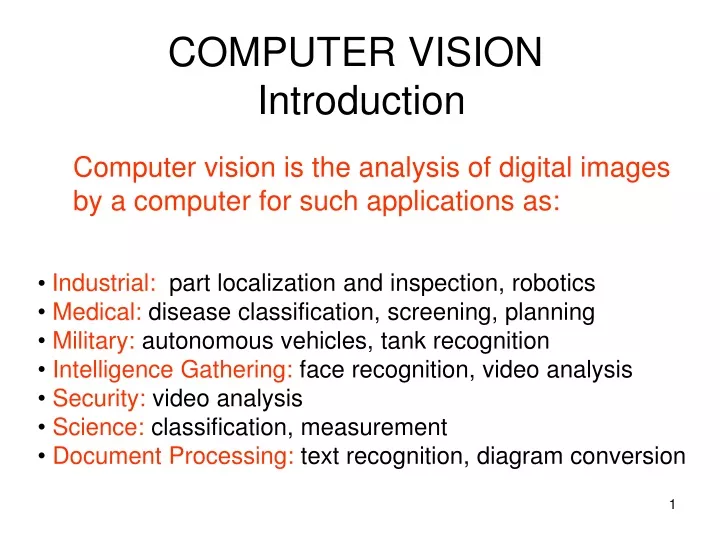
1. COMPUTER VISION Introduction Computer vision is the analysis of digital images by a computer for such applications as: • Industrial: part localization and inspection, robotics • Medical: disease classification, screening, planning • Military: autonomous vehicles, tank recognition • Intelligence Gathering: face recognition, video analysis • Security: video analysis • Science: classification, measurement • Document Processing: text recognition, diagram conversion

2. The Three Stages of Computer Vision • low-level (image processing) • mid-level (feature extraction) • high-level (the intelligent part) image image image features features analysis

3. Low-Level Canny edge operator original image edge image Mid-Level (Lines and Curves) ORT line & circle extraction data structure circular arcs and line segments edge image

4. Low- to High-Level low-level edge image mid-level consistent line clusters high-level BuildingRecognition

5. Mid-level (Regions) K-means clustering (followed by connected component analysis) original color image regions of homogeneous color data structure

6. Image Databases: Images from my Ground-Truth collection. • Retrieve all images that have trees. • Retrieve all images that have buildings. • Retrieve all images that have antelope.

7. Simpler • Retrieve images based on their color and texture attributes • Color histograms • Texture histograms • Both • This is content-based image retrieval: CBIR.

8. standard for cameras hue, saturation, intensity intensity plus 2 color channels color TVs, Y is intensity • RGB • HSI/HSV • CIE L*a*b • YIQ • and more Color Spaces

9. RGB Color Space Absolute Normalized Normalized red r = R/(R+G+B) Normalized green g = G/(R+G+B) Normalized blue b = B/(R+G+B) (0,0,255) R,G,B) blue (0,0,0) (0,255,0) red green (255,0,0)

10. Conversion from RGB to YIQ An approximate linear transformation from RGB to YIQ: We often use this for color to gray-tone conversion.

11. Histograms • A histogram of a gray-tone image is an array H[*] of bins, one for each gray tone. • H[i] gives the count of how many pixels of an image have gray tone i. • P[i] (the normalized histogram) gives the percentage of pixels that have gray tone i.

12. Color histograms can represent an image • Histogram is fast and easy to compute. • Size can easily be normalized so that different image histograms can be compared. • Can match color histograms for database query or classification.

13. Histograms of two color images

14. How to make a color histogram • Make a single 3D histogram. (BIG) • Make 3 histograms and concatenate them. (Most Common and what Bindita has) • Create a single pseudo color between 0 and 255 by using 3 bits of R, 3 bits of G and 2 bits of B (Old) • Use normalized color space and 2D histograms.

15. Apples versus Oranges H S I Separate HSI histograms for apples (left) and oranges (right) used by IBM’s VeggieVision for recognizing produce at the grocery store checkout station (see Ch 16).

16. Skin color in RGB space (shown as normalized red vs normalized green) Purple region shows skin color samples from several people. Blue and yellow regions show skin in shadow or behind a beard.

17. Finding a face in video frame • (left) input video frame • (center) pixels classified according to RGB space • (right) largest connected component with aspect similar to a face (all work contributed by Vera Bakic)

18. (from Swain and Ballard) 3D color histogram cereal box image

19. Four views of Snoopy Histograms

20. Uses • Although this is an extremely simple technique, it became the basis for many content-based image retrieval systems and works surprisingly well, both alone, and in conjunction with other techniques.

21. Texture • Color is well defined. • But what is texture?

22. Structural Texture Texture is a description of the spatial arrangement of color or intensities in an image or a selected region of an image. Structural approach: a set of texels in some regular or repeated pattern

23. Natural Textures from VisTex grass leaves What/Where are the texels?

24. The Case for Statistical Texture • Segmenting out texels is difficult or impossible in real images. • Numeric quantities or statistics that describe a texture can be computed from the gray tones (or colors) alone. • This approach is less intuitive, but is computationally efficient. • It can be used for both classification and segmentation.

25. Some Simple Statistical Texture Measures Edge Density and Direction • Use an edge detector as the first step in texture analysis. • The number of edge pixels in a fixed-size region tells us how busy that region is. • The directions of the edges also help characterize the texture

26. Example Original Image Frei-Chen Thresholded Edge Image Edge Image

27. Local Binary Pattern Measure • For each pixel p, create an 8-bit number b1 b2 b3 b4 b5 b6 b7 b8, where bi = 0 if neighbor i has value less than or equal to p’s value and 1 otherwise. • Convert these 8-bit strings to integers. • Represent the texture in the image (or a region) by the histogram of these numbers. 1 2 3 100 101 103 40 50 80 50 60 90 4 5 1 1 1 1 1 1 0 0 8 252 7 6

28. Distance Measures • In order to retrieve images from a database, we need to use distance measures to measure how far is a query image from each database image. • The most common distance measure in a vector space is Euclidean Distance. • D((x1,x2,…xn),(y1,y2,…yn)) = sqrt[(x1-y1)2 + (x2-y2)2 + … +(xn-yn)2] • HW4 asks you to use this plus 3 others.

29. Example Fids (Flexible Image Database System) is retrieving images similar to the query image using LBP texture as the texture measure and comparing their LBP histograms

30. Example Low-level measures don’t always find semantically similar images.

31. What else is LBP good for? • We found it in a paper for classifying deciduous trees. • We used it in a real system for finding cancer in Pap smears. • We are using it to look for regions of interest in breast and melanoma biopsy slides. • You will use it for HW4.

32. CSE 473 Winter 2019 Homework 4 Content-based Image Retrieval

33. Introduction • Given a database of images (40 images belonging to 8 classes with 5 images per class) and a query image, retrieve the images from the database which are most similar to the query image. • In python, an image with height H, width W and number of channels C (3 for RGB images) is represented by a 3D matrix of shape H x W x C. • To access a particular pixel (h,w) of a particular channel (c) of the 'image' variable, use image[h,w,c] • Write your code in the code file (main.py) and your comments and results on the Overleaf (Latex) document as a report (main.pdf). Submit these 2 files.

34. Overleaf

35. Instructions • Compute a feature vector for each image. Use two types of features: • Color Histogram: Compute 3 variations • histogram with grayscale values and 8 bins • histogram with grayscale values and 256 bins • histogram with RGB values and n bins, where n depends on which of the above 2 you found better • LBP (Local Binary Pattern) Histogram: Compute 2 variations • histogram from the entire image • histogram by concatenating histograms from each 16x16 region

36. Instructions • Use a distance measure to compare the feature vectors and retrieve images in the order of increasing distance (images with lesser distance values are more similar to the query image) • Compare different distance measures as asked in the report. • To run the starter code, open your terminal in the homework folder and type: • $ python main.py -q beach_1 • Further instructions are written in the starter code. • Questions are directly written in the report. Write your solutions where asked.

37. Sample (random) output for query beach_1