Download
1 / 62
1.23k likes | 2.29k Views
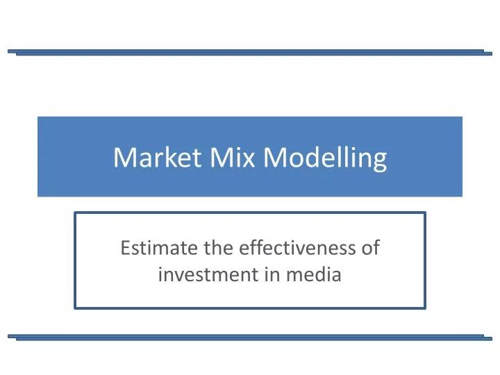
Market Mix Modelling. Estimate the effectiveness of investment in media. Agenda. Business application of Marketing Mix modelling A case study Strengths and weaknesses Brief introduction to more advanced approaches: pooled regressions and structural equations.

E N D
Market Mix Modelling Estimate the effectiveness of investment in media
Agenda • Business application of Marketing Mix modelling • A case study • Strengths and weaknesses • Brief introduction to more advanced approaches: pooled regressions and structural equations
Making BP’s media dollars work harder • “Mindshare helped BP to make the most of their media investments across the many states of the USA.” • “BP engaged Mindshare to develop enhanced media investment strategies to maximise sales and boost revenue performance.” • “Drivers of performance were quantified (e.g. media, promotions, distribution, competitor effects) in seven USA states, over three years” • “Return on investment figureswere calculated - both short and long term - for 40 campaigns.”
Marketing Mix modelling • Statistical methods applied to measure the impact of media investments, promotional activities and price tactics on sales or brand awareness • Used to assist and implement a marketing strategy by measuring: • Effectiveness: contribution of marketing activities to sales • Efficiency: short term and long term Return-On-Investment of marketing spend • Price elasticity • Impact of competitors
MMM How does it work? • A statistical model is estimated on historical data with sales as a dependent variable and list of explanatory variables as marketing activities, price, seasonality and macro factors • The simplest and broadly used model is linear regression: • The output of the model is then used to carry out further analysis like media effectiveness, ROI and price elasticity and to simulate what-if scenarios
Factors that could drive sales Advertising TV Radio Print Outdoor Internet Promotions Sponsorships Events Price Adv quality Distribution Merchandising Competition Seasonality Weather Economic Demographic Industry data Sales
MMM project process • Set out objectives • Define scope • Discuss data availability • Design data-warehouse • Data preparation • Collect data • Validate, harmonize and consolidate data • Present exploratory analysis to client • Presentation • Interpretation of results • Learning and recommendations • Model development • Estimation • Diagnostics • Calculate ROIs, Price elasticity and response curves
Case study • An energy company SPetrol wants to evaluate the advertising investments of its retail business in the US from 2001 until 2004. • Client’s questions: • How much have we made through advertising? • What is the return on investments of our media activities? • Which marketing drivers have had the greatest effect? • What’s the influence of price on our sales? • Are we optimally allocating our budget across products ?
Advertising data • The performance of TV and radio advertising is expressed in terms of Gross Rating Points (GRPs) . A rating point is a percentage of the potential audience and GRPs measure the total of all rating points during and advertising campaign. • GRPs (%) = Reach * Frequency • Example: Let’s assume a commercial is broadcasted two times on TV GRPs 57% 1st time on air 25% of target televisions are tuned in 2st time on air 32% of target televisions are tuned in
Advertising data • Spetrol has deployed 5 TV campaigns over the sample with a total expenditure of 300 million $ • Each campaign lasted from 4 to 8 weeks • Is there any relationship between sales and TV advertising?
Carry over effect of TV • The exposure to TV advertising builds awareness, resulting in sales. • ADStock allows the inclusion of lagged and non linear effects • Alpha is estimated iteratively using least squares. The estimate is then validated by media planners
Advertising data 300 M TV Spend 164 M Radio 160 M Outdoor
Below the line promotions • It may include • sponsorship • product placement • sales promotion • merchandising • trade shows • Usually represented by dummies (variables equal to 1 when a promotion takes place and 0 otherwise)
Below the line promotions Sponsorship World Rally Championship Sale promotion Sale promotion 5% Discountt
Seasonality August seasonal dummy Peaks every year in August Sale promotion 5% Discountt
Exploratory analysis Scatter plot Unit root test Histogram and desc stats Correlation matrix
Estimated equation Salest = 167412+ 168* AdStock(GRPsTVt,0.75) + 161* AdStock(GRPsRadiot,0.35) + 166* AdStock(Outdoort,0.15) + 580* PromotionDummyt + 6507* Seasonalityt + -12631* Pricet + Errort
Model diagnostics • Model: • Significant F-stat and high R-squared • Variables: • Significant T-stats • Coefficients must make sense • Variance inflation factor low • Residuals: • Normality (Jarque-Bera) • Absence of serial correlation ( Durbin Watson, correlogram)
Residuals diagnostics • Durbin Watson = 1.69 • DW>2 positive autocorrelation • DW<2 negative autocorrelation
Estimated factors contribution to sales • Fitted Salest = estimated Intercept = 167,412 • Can be interpreted as Brand Equity: • Volume generated in absence of any marketing activity • Indicator of the strength of the brand and users’ loyalty
Estimated factors contribution to sales TV Contributiont(000’ Gallons) = coefficient *Adstock(TV)t • Fitted Salest = 167,412 + 168* TVt + 161*Radiot+ • 166*OOHt+ 580* Promotiont
Estimated factors contribution to sales Peacks every year in August Peaks every year in August • Fitted Salest = 167,412 + 168* TVt + 161*Radiot+ • 166*OOHt+ 580* Promotiont + 6507* Seasonailityt Equity = estimated Intercept = 167,412 Can be interpreted as Brand Equity
Estimated factors contribution to sales Fitted Salest = 167,412 + 168* TVt + 161*Radiot+ 166*OOHt+ 580* Promotiont + 6507* Seasonailityt - 12631* Pricet Negative price effect
Does it really make sense? The more I invest in media, the more I sell Diminishing returns
Response curves Taking into account diminishing returns
Price elasticity • Assumption: constant elasticity across the sample which implies a linear relation between volume and price • By using the coefficient of the regression, it is possible to derive an estimate for price elasticity: • Price coefficient = -12631 • Average price = 1.51 $ • Average volume sales = 154,000 Gallons A 10% drop in price increases sales by 1.2%
Dynamic price elasticityElasticity changes with price Estimated through non linear regressions Elastic (>1): Demand is sensitive to price changes. Inelastic (<1): Demand is not sensitive to price changes
Client’s questions How much have we made through advertising? • 1 billion $ driven by TV • 500 million $ due to radio • 200 million $ generated by Outdoor and promotional activities • Investments in media generated 1.7 billion $ in revenue
Client’s questions What is the return on investments of our media activities? For each dollar invested in TV you get 3.5 dollars back
Client’s questions What’s the influence of price on our sales? A 10% drop in price increases sales by 1.2%
Maximum Marginal Return Point of Saturation Maximum Average Return Are we optimally allocating our budget across products ? Optimal GRPs Over Optimal GRPs Sub –Optimal GRPs Invest more in Radio and less in OOH
5000 4500 4000 Promo TV Saturation 3500 3000 Weekly Sales Current 2500 Optimal 2000 1500 1000 500 0 0 20 40 60 80 100 120 140 160 180 Avg. Weekly GRPs Marketing Mix – Sample Output Marketing mix (sample output) 45 Carry Over Effect Diminishing Returns 40 35 30 25 Weekly GRPs 20 15 10 5 0 Diminishing Returns is the point were spending additional GRPs does not results in additional sales.Carry Over Effect (Ad Stock) relates to the residual effect of an ad.When all the components are layered on Base sales, it is clear what drivers contribute to sales and when and their Simultaneous Effect. Week1 Week2 Week3 Week4 Week5 Simultaneous Effect Volume Base/Seasonal TV/Radio/Print Direct Marketing Rates/Promotions Time
Pros and cons • Simple and intuitive • The outcome is backed by qualitative expertise and in field research • Constructive way of running different scenarios and evaluating past performance • Better with granular data • Very successful method – high turnover • Correlation doesn’t imply causality • Risk of spurious regressions especially when modelling in levels • Model highly depends on variables chosen • Poor in forecasting
Spurious statistics • A high correlation between sales and TV could mean: • Either media causes sales • or sales causes media • or a third variable causes both sales and TV Sales Media Income What is the truth?
Non sense correlations • Some spurious correlations: • death rate and proportion of marriages Corr =0.95 • National income and sunspots Corr =0.91 • Inflation rate and accumulation of annual rainfall • On the other hand, a low correlation doesn’t rule out the possibility of a strong relation: Corr = 0.0 • Correlations must support a theory • Calculate correlations both in levels and differences • Always look at scatter plots