Download
1 / 28
280 likes | 548 Views
Property Taxation in Michigan. Mark Skidmore Morris Chair in State and Local Government Finance and Policy Presented at: “Economic Health and Public Finance in Michigan” October 6-7, 2008. Presentation Outline. Key features of the property tax Interactions with other policies

E N D
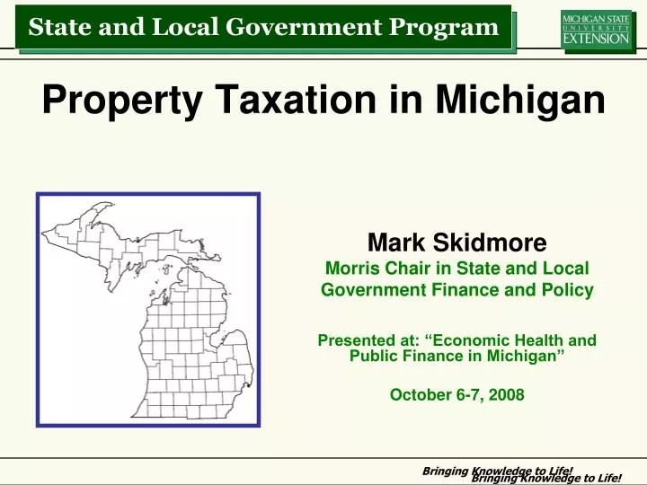
Property Taxation in Michigan Mark Skidmore Morris Chair in State and Local Government Finance and Policy Presented at: “Economic Health and Public Finance in Michigan” October 6-7, 2008
Presentation Outline • Key features of the property tax • Interactions with other policies • Taxable value cap, falling home values, and foreclosure • Taxable value cap, tax base erosion and tax burden distribution • Conclusions
Features of the Property Tax • Headlee amendment implemented in 1978 • Growth in property tax revenues cannot exceed the rate of inflation plus taxes generated from new construction • If the value of existing property exceeds the limit, a rate rollback is required. (Headlee rollback) • Prior to 1994, rollbacks were fairly common…rollbacks were applied to all properties in the jurisdiction. • Michigan is not alone in implementing such limitations, and research shows that such constraints limit property tax revenue growth. • Special assessments (levied without voter approval, not subject to constitutional limits • Finance street improvements, sewer, police, fire, trash collection • Mobile home park exemption
Proposition A • Proposition A was implemented in 1994 • Professor Papke will cover education spending policy on Tuesday. I focus on the property tax changes. • Cut homestead millage rates • Cut statewide average school millage rates from 34 mills to 6 mills (state education tax) • 18 mill limit for schools on non-homestead property • Increased the cigarette tax • Increased the sales tax rate • *Placed a constitutional cap on the growth of assessment increases for tax purposes
Proposition A • The taxable value of a property is allowed to increase by the lesser of the rate of inflation or 5%. • Historically, taxable value (TV) grew less slowly than state equalized value (SEV) • Growth in TV < Growth in SEV so that (TV/SEV)↓ • Tax Base Erosion • A couple rules • TV increases to SEV when a home is sold (“pop up”) • For new construction, TV = SEV • Applies to each individual property, not a jurisdiction’s in aggregate property values • Growth in SEV and TV depend on: • The rate of property turnover • The rate of new construction • The rate of growth (or decline) in actual property values
Ratio of taxable value to state equalized value: 2008 Legend 57.0% - 62.7% 62.7% - 68.7% 68.7% - 73.5% 73.5% - 79.3% Greater than 79.3% TV/SEV by Property Type • Statewide Tax • Base Erosion • YearTV/SEV • 1994 1.00 • 0.77 • 0.78 • 2008 0.81 Source: Michigan Department of Treasury
Interactions with Other Policies • Income tax • Circuit-breaker property tax credit available: • available to those with income under $82,650 and • if property taxes exceed 3.5% of income • Over the age of 65—100% credit on income taxes • Under the age of 65—the credit depends on income level • phased out as income increases • Professor Menchik discussed the circuit-breaker and other preferential income tax treatments
Interactions with Other Policies • Education finance (Papke) • Tax abatement programs (Sands) • Such programs may serve to spur development in designated areas, BUT there is a cost: • Hold public services/spending constant, others pay more taxes
Falling Home Values, Foreclosure and Property Tax Revenues • Falling home values and foreclosure reduce the tax base • Under the taxable value cap, tax base reductions have short-run and long-run implications • Short-run: Insulates local revenues from the declining home values • Long-run: Leads to significant fiscal challenges
Housing Prices • Housing prices will continue to fall if we are to return to historical trend.
Property Values • The motivation behind the assessment growth limit was to protect property owners from “excessive” growth in property taxes due to increasing property values. • Falling home values was unanticipated. • Consider the following graph to understand the implications…
Tax Payment with Falling Home Values • What if SEV falls below TV for a particular property? • Assessors increase TV by the rate of inflation even in the face of falling housing prices….until TV=SEV. • Then TV follows SEV. • When house prices stabilize and begin to increase, TV is ratcheted down….local unit fiscal capacity may not recover for years.
Implications for Local Government Fiscal Health • Under the taxable value cap, local government fiscal capacity (especially in areas of significant housing price declines) may be severely curtailed for years to come. • The taxable value cap constrains property tax revenue recovery • Housing values will eventually recover, but taxable values are only allowed to grow at the rate of inflation • Extend fiscal problems…unless voters support a rate increase via referenda processes
Tax Burden Redistribution under the Taxable Value Cap • If all property value were taxed fully, statewide average statutory property tax rates could fall by about 19 percent. • Long-time homeowners who experienced housing price appreciation received tax relief. • Recent home buyers experience a tax penalty.
Property Tax Burden • Anyone who has recently bought a home understands this • The tax payment of the previous owner does not necessarily reflect what you will pay when you purchase the home • The previous owner’s tax payment was based on the taxable value • Your payment is based on state equalized value (the “pop up” effect)
Property Tax Burden • Little is known about how property tax burdens have been redistributed across socio-economic groups • Using the State of the State Survey (administered by MSU), Ballard, Hodge, and Skidmore are in the process of evaluating this issue • roughly 1,000 respondents on the survey • Detailed economic and demographic information • Questions on property tax payments and perceived home values • Match survey data with community-level data
Property Tax Burden • What are the tax savings associated with length of tenure in a home? • What demographic characteristics are associated with length of tenure in a home? • Which demographic groups have benefited (or been hurt) by the taxable value cap?
Property Tax Burden • Calculate effective tax rates for each homeowner in the survey • Identify the determinants of effective tax rates • The difference between statutory rates and effective tax rates: • - Statutory Rate = Tax Payment/Taxable Value • - Effective Rate = Tax Payment/State Equalized Value
Property Tax Burden • Community Characteristics: • population • per capita state equalized value in community (wealth) • urban indicator defined by Census • city indicator (as opposed to township) • Detroit indicator (very high statutory rates) • mobile home park indicator (no tax) • Years • Years of tenure in a home
Property Tax Burden • On average, for every year a person owns a home, property tax rates (and tax payments) are reduced by 0.34 millage points relative to a person who recently purchased a home. • Since 1994—tax savings accrues to nearly 5 millage points or about 17% over new homeowners. • For communities defined as “rural” there is a 20% differential. • For communities with populations between 10,000 and 40,000, this differential is about 45%.
Property Tax Burden • Consider socio-economic characteristics • What characteristics are potentially correlated with length of tenure in a home? • Age* • Income • Race (average length of tenure is about 6 years less for African Americans than for Caucasians) • Other socio-economic characteristics
Property Tax Burden • AGE • - On average, tax savings accrue by 0.16 millage points for each year of age (estimates vary depending on location) • - Average tax savings for a 63 year old over a 23 year old is about 16% annually, controlling for other factors • Other findings: • As income, rises effective tax rates fall slightly • Controlling for age, race has no bearing on tax burden
Conclusions • The taxable value cap was perceived to be a tax relief measure (above and beyond the Headlee amendment) • Falling home values was unanticipated • Significant long-term fiscal stress will likely result under the current legal environment • Distributional consequences unanticipated • One average, older high income homeowners have benefited…at the expense of younger lower income homeowners
Conclusions • One might argue that because home values are falling, the distribution issue is no longer relevant • BUT now is a excellent time to seek its repeal • With falling home values, long-time homeowners have less to lose by repeal than in previous years • Voter approval is required • Other research shows that such restrictions reduce mobility (“lock in effect”)
Conclusions • Repeal of the taxable value cap would • Reduce statewide average statutory rates by 19% • Eliminate differences in effective tax rates across owners of equivalently valued homes • Reduce rates for new homeowners • Increase rates of long-time homeowners (with no impact on the low to moderate income elderly…circuit-breaker) • Eliminate any “lock-in” effects • Reduce rates for new businesses not already receiving tax abatements, and raise rates of long-time existing businesses • Provide local (and state) officials with more flexibility in managing fiscal challenges in the coming years • Circuit-breakers still protect elderly and low/moderate income homeowners