Download
1 / 57
570 likes | 585 Views
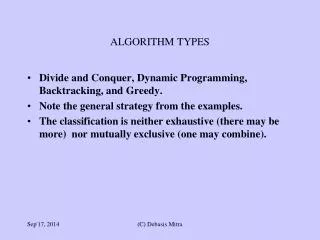
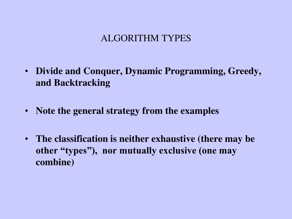
ALGORITHM TYPES. Divide and Conquer, Dynamic Programming, Greedy, and Backtracking Note the general strategy from the examples The classification is neither exhaustive (there may be other “types”), nor mutually exclusive (one may combine). Divide and conquer: Solves a problem top-down

E N D
ALGORITHM TYPES Divide and Conquer, Dynamic Programming, Greedy, and Backtracking Note the general strategy from the examples The classification is neither exhaustive (there may be other “types”), nor mutually exclusive (one may combine)
Divide and conquer: Solves a problem top-down Dynamic Programming: Bottom-up DP starts with Recurrence Eq. Recursive: with possibility of repeatedly computing same Compute the smaller components and keep combining them Then, bottom up approach Save and reuse intermediate results in a data structure Space traded off for time DYNAMIC PROGRAMMING STRATEGY: BIG PICTURE
Bottom up approach for computing a Recurrence Save and reuse intermediate results in a data structure Space traded off for time Fibonacci-series calculation: f(n) = f(n-1) + f(n-2), for n>1; f(0)=f(1)=1 n = 1, 2, 3, 4, 5 fib = 1, 2, 3, 5, 8 Draw the recursion tree of Fibonacci-series calculation, you will see example of such repetitive calculations PROBLEM 0: DYNAMIC PROGRAMMING STRATEGY
DYNAMIC PROGRAMMING STRATEGY (Continued) Recursive fibonacci(n) if (n<=1) return 1; else return (fibonacci(n-1) + fibonacci(n-2)). Time complexity: exponential, O(kn) for some k>1.0 Iterative fibonacci(n) fib(0) = fib(1) = 1; for i=2 through n do fib(i) = fib(i-1) + fib(i-2); end for; return fib(n). Time complexity: O(n), Space complexity: O(n)
SpaceSaving_fibonacci(n) if (n<=1) return 1; int last=1, last2last=1, result=1; for i=2 through n do result = last + last2last; last2last = last; last=result end for; return result. Time complexity: O(n), Space complexity: O(1) DYNAMIC PROGRAMMING STRATEGY (Continued)
In fib(5) recursive call recalculates fib(1) 5 times, fib(2) 3 times, fib(3) 2 times. The complexity is exponential. Iterative calculation avoids repetition: stores the needed values in variables - complexity linear O(n) Dynamic Programming typically consumes more memory to store the result of calculations of lower levels for the purpose of calculating the next higher level. Intermediate results are typically stored in atable. DYNAMIC PROGRAMMING STRATEGY (Continued)
Given a set of objects with (Weight, Profit) pair, and a Knapsack of limited weight capacity (M), find a subset of objects for the knapsack to maximize total profitP Sample Problem: Objects (wt, p) = {(2, 1), (3, 2), (9, 20), (5, 3)}. M=8 Exhaustive Algorithm: Try all subset of objects. How many? Problem 2: 0-1 Knapsack Problem (not in the book) {}: total=(0 lbs, $0) {(2,1)}: total =(2lbs, $1) … {(9,20): Illegal, total wt>8 … {(2,1), (3,2)}: =(5lbs, $3) … Total possibilities = 2n For each object present or absent 0 or 1 A bit string is a good representation for a set, e.g. 000101100…. n-bits
Formulate a recurrence for optimal profit P(j, k): for the first j objects considered (in any arbitrary but pre- ordering of objects) with a variable knapsack limit k Develop the table for P(j, k) with rows j =1 …n (#objects), and for each row, go from k =0 …M (the KS limit) Finally P(n, M) gets the result 0-1 Knapsack Problem P(j, k): k j |
0-1 Knapsack Recurrence Formula for computing P • The recurrence, for all k=0…M, j=0…N P(j, k) = (case 1) P(j-1, k), if wj>k, wj is weight of the j-th object; else P(j, k) = (case2) max{ P(j-1, k-wj)+pj, P(j-1, k) } • Explanation for the formula is quite intuitive • Recurrence terminates: P(0, k)=0, P(j, 0)=0, for all k’s and j’s Objects (wt, p) = {(2, 1), (3, 2), (5, 3)}. M=9
Recurrence -> recursive algorithm Input: Set of n objects with (wi, pi) pairs, and knapsack limit M Output: Maximum profit P for subset of objects with total wt ≤ M Function P(j, k) • If j ≤ 0 or k ≤ 0 then return 0; //recursion termination • else • if wj>k then • return P(j-1, k) // recursive call • else • return max{P(j-1, k-Wj) + pj, P(j-1, k)} // recursive call End algorithm. Driver: call P(n, M), for given n objects & KS limit M. This is not table building: P’s are recursive functions Complexity: ? Exponential: O(2n) Why? Same reason as in Fibonacci number calculation: Repeats computing intermediate P’s
0-1 Knapsack: Recursive call tree Objects (wt, p) = {(2, 1), (3, 2), (5, 3)}. M=8 P(3,8) P(2,8-5) P(2,8) P(1,3-3) P(1,8-3) P(1,3) P(1,8) w1 =2>0, not called P(0,8) P(0,8-2) P(0,3-2) P(0,3) P(0,5-2) P(0,5) P(0,0-2) P(0,0) Each leaf has w=0, and P(0,*) returns a value, 0 to the caller above
0-1 Knapsack: recurrence -> DP algorithm Do not repeat the same computation, store them in a table and reuse Input: Set of n objects with (wi, pi) pairs, and knapsack limit M Output: Maximum profit P for a subset of objects with total_wt ≤M Algorithm DPks(j, k) • For all k, P(0, k) =0; For all j, P(j, 0) = 0; // initialize MATRIX P(j, k) • For j=1 to n do • For k= 1 to M do • if wj>k then • P(j, k) = P(j-1, k) • else • P(j, k)= max{P(j-1, k-Wj) + pj, P(j-1, k)} End loops and algorithm Complexity: O(nM), pseudo-polynomial because M is an input value. If M=30.5 the table would be of size O(10nM), or if M=30.54 it would be O(100NM).
0-1 Knapsack Problem (Example) Objects (wt, p) = {(2, 1), (3, 2), (5, 3)}. M=8 +2$ +0$ -5 lbs (2+3)$
What if M=9 Objects (wt, p) = {(2, 1), (3, 2), (5, 3)}. M=9 -5 lbs (2+3)$ HOW TO FIND KNAPSACK CONTENT FROM TABLE? SPACE COMPLEXITY?
Memoisation algorithm: 0-1 knapsack Algorithm P(j, k) If j <= 0 or k < = 0 then return 0; // recursion termination else if Wj>k then y=A(j-1, k); if y<0 {y = P(j-1, k) ; A(j-1, k)=y}; // P( ) is a recursive call, A( ) is matrix return y else x=A(j-1, k-Wj); if x<0 {x = P(j-1, k-Wj) ; A(j-1, k-Wj)=x}; y=A (j-1, k); if y<0 {y = P(j-1, k) ; A(j-1, k)=y}; A (j, k) = max{x+ pj, y}; return max{x+ pj, y} End algorithm. Driver: Initialize global matrix A(0->n, 0->M)= -1; call P(n, M) Complexity: best of the both recursive and DP algorithms, but …?
A chain of matrices to be multiplied: ABCD, dimensions: A (5x1), B(1x4), C(4x3), and D(3x6). Resulting matrix will be of size (5x6). # scalar (or integer) multiplications for (BC) is 1.4.3, and the resulting matrix’s dimension is (1x3), 1 column and 3 rows. Problem 2: Ordering of Matrix-chain Multiplications
Ordering of Matrix-chain Multiplications A (5x1), B(1x4), C(4x3), and D(3x6) • Multiple ways to multiply: • (A(BC))D, • ((AB)C)D, • (AB)(CD), • A(B(CD)), • A((BC)D) • note: Resulting matrix would be the same • but the computation time may vary drastically • Time depends on #scalar multiplications • In the case of (A(BC))D, it is = 1.4.3 + 5.1.3 + 5.3.6 = 117 • In the case (A(B(CD)), it is = 4.3.6 + 1.4.6 + 5.1.6 = 126 • Our problem here is to find the best such ordering • An exhaustive search over all orderings is too expensive - Catalan number involving n!
For a sequence A1...(Aleft....Aright)...An, we want to find the optimal break point for the parenthesized sequence. Calculate for ( r-l+1) number of cases and find the minimum: min{(Al...Ai) (Ai+1... Ar), with li< r}, Recurrence for optimum scalar-multiplication: M(l, r) = min{M(l, i) + M(i+1, r) + rowl .coli .colr, with li < r}. Termination: M(l, l) = 0 Recurrence for Ordering of Matrix-chain Multiplications r = 1 2 3 4 lft 1 0 15 35(2) 69(2) 2 0 12 42 3 0 24 4 0 Sample M(i,j):
Matrix-chain Recursive algorithm Recursive Algorithm M(l, r) • if r<= l then return 0; // Recurrence termination: no scalar-mult • else • return min{M(l, i) + M(i+1, r) + rowl.coli .colr , • for li<r}; • end algorithm. Driver: call M(1, n) for the final answer.
Recurrence for optimum scalar-multiplication: M(l, r) = min{M(l, i) + M(i+1, r) + rowl.coli .colr, with li < r}. To compute M(l,r), you need M(l,i) and M(i+1,r) available for ALL i’s E.g., For M(3,9), you need M(3,3), M(4,9), and M(3,4), M(5,9), … Need to compute smaller size M’s first Gradually increase size from 1, 2, 3, …, n Recurrence for Ordering of Matrix-chain Multiplicationsto Bottom-up Computation
Recurrence for optimum number of scalar-multiplications: M(l, r) = min{M(l, i) + M(i+1, r) + rowl .coli .colr , with li < r}. Compute by increasing size: r-l+1=1, r-l+1=2, r-l+1=3, … r-l+1=n Start the calculation at the lowest level with two matrices, AB, BC, CD etc. Really? Where does the recurrence terminate? Then calculate for the triplets, ABC, BCD etc. And so on… Strategy for Ordering of Bottom-up Computation =0, for l==r
r = 1 2 3 4 l 1 0 15 35(2) 69(2) 2 0 12 42 3 0 24 4 0 Ordering of Matrix-chain Multiplications (Example) Triplets Pairs Singlet's
Matrix-chain DP-algorithm Input: list of pairwise dimensions of matrices Output: optimum number of scalar multiplications • for all 1i n do M(i,i) = 0; //diagonal elements 0 • for size = 2 to n do // size of subsequence • for l =1 to n-size+1 do • r = l+size-1; //move along diagonal • M(l,r) = infinity; //minimizer • for i = l to r-1 do • x = M(l, i) + M(i+1, r) • + rowl.coli .colr; • if x < M(l, r) then M(l, r) = x; End. // Complexities?
r = 1 2 3 4 l 1 0 2 0 3 0 4 0 Ordering of Matrix-chain Multiplications (Example) A1 (5x3), A2(3x1), A3 (1x4), A4 (4x6). 15 35(2) 69(2) 12 42(?) 24 Triplets Pairs How do you find out the actual matrix ordering? Calculation goes diagonally. COMPLEXITY?
A1 (5x3), A2 (3x1), A3 (1x4), A4 (4x6). M(1,1) = M(2,2) = M(3,3) = M(4,4) = 0 M(1, 2) = M(1,1) + M(2,2) + 5.3.1 = 0 + 0 + 15. M(1, 3) = min{i=1 M(1,1)+M(2,3)+5.3.4, i=2 M(1,2)+M(3,3)+5.1.4 } = min{72, 35} = 35(2) M(1,4) = min{ i=1 M(1,1)+M(2,4)+5.3.6, i=2 M(1,2)+M(3,4)+5.1.6, i=3 M(1,3)+M(4,4)+5.4.6} = min{132, 69, 155} = 69(2) 69 comes from the break-point i=2: (A1.A2)(A3.A4) Recursively break the sub-parts if necessary, e.g., for (A1A2A3) optimum is at i=2: (A1.A2)A3 DP Ordering of Matrix-chain Multiplications (Example)
r = 1 2 3 4 l 1 0 15 35(2) 69(2) 2 0 12 42 3 0 24 4 0 Ordering of Matrix-chain Multiplications (Example) A1 (5x3), A2 (3x1), A3 (1x4), A4 (4x6). Triplets Pairs For a chain of n matrices, Table size=O(n2), computing for each entry=O(n): COMPLEXITY = O(n2 *n) = O(n3) A separate matrix I(i,j) keeping track of optimum i, for actual matrix ordering
Computing the actual break points I(i,j) r = 1 2 3 4 5 6 l 1 - - (2) (2) (3) (3) 2 - - (3) (3) (4) 3 - - (4) (4) 4 - (3) (4) 5 - - - 6 - - - Backtrack on this table: (A1..A3)(A4…A6) ABCDEF -> (ABC)(DEF) Then: (A1..A3) -> (A1A2)(A3), & (A4…A6) -> A4(A5 A6) ABCDEF -> (ABC)(DEF) -> ((AB)C) (D(EF))
Inductive Proof of Matrix-chain Recurrence Induction base: • if r< l then absurd case, there is no matrix to multiply: return 0; • If r = = l, then only one matrix, no multiplication: return 0 Inductive hypothesis: • For all size<k, and k≥1, assume M(l,r) returns correct optimum Note: size = r-l+1 Inductive step, for size=k: • Consider all possible ways to break up (l…r) chain, for l i<r : • Make sure to compute and add the resulting pair of matrices multiplication: rowl.coli .colr • Since M(l,i) and M(i+1,r) are correct smaller size optimums, as per hypothesis, min{M(l, i) + M(i+1, r) + rowl.coli .colr , for li<r} is the correct return value for M(l,r)
Be careful with the correctness of the Recurrence behind Dynamic Programming Inductive step: • Consider all possible ways to break up (l…r) chain, for li<r : • Make sure to compute the resulting pair of matrices multiplication: rowl.coli .colr • Since M(l,i) and M(i+1,r) are correct smaller size optimums, per hypothesis, min{M(l, i) + M(i+1, r) + rowl.coli .colr , for li<r} is the correct return value for M(l,r) It is NOT always possible to combine smaller steps to the larger one. Addition, Multiplication are associative: 4+3+1+2+9 = (((4+3) +(1+2)) +9) , but average(4,3,1,2,9) = av( av(av(4,3), av(1,2)), 9), NOT true • DP needs the correct formulation of a Recurrence first, • Then, bottom up combination such that smaller problems contributes to the larger ones
Problem 3: Optimal Binary Search Tree Binary Search Problem: Input: sorted objects, and key Output: the key’s index in the list, or ‘not found’ Binary Search on a Tree: Sorted list is organized as a binary tree Recursively: each root t is l ≤t ≤r, where l is any left descendant and r is any right descendant Example sorted list of objects: A2, A3, A4, A7, A9, A10, A13, A15 Sample correct binary-search trees: A1 A7 A3 A4 A10 A3 A7 A9 A13 A2 A4 A9 A10 A13 A15 A15 There are many such correct trees
Problem 3: Optimal Binary Search Tree Problem: Optimal Binary-search Tree Organization Input: Sorted list, with element’s access frequency (how many times to be accessed/searched as a key over a period of time) Output: Optimal binary tree organization so that total cost is minimal Cost for accessing each object= frequency*access steps to the object in the tree) Number of Access steps for each node is its distance from the root, plus one. Example list sorted by object order (index of A): A1(7), A2(10), A3(5), A4(8), and A5(4) A1(7) A3(5) A2(10) A3(5) A4(8) A1(7) A4(8) A5(4) A2(10) A5(4) Cost = 5*1 + 7*2 + 10*3 + 8*2 + 4*3 = 77 Cost = 7*1 + 10*2 + 5*3 + 8*4 + 4*5 =94
Problem 3: Optimal Binary Search Tree Input: Sorted list, with each element’s access frequency (how many times to be accessed/searched as a key over a period of time) Output: Optimal binary tree organization with minimal total cost Every optimization problem optimizes an objective function: Here it is total access cost Different tree organizations have different aggregate costs, because the depths of the nodes are different on different tree. Problem: We want to find the optimal aggregate cost, and a corresponding bin-search tree.
Problem 3: Optimal Binary Search Tree Step 1 of DP: Formulate an objective function For our example list: A1(7), A2(10), A3(5), A4(8), and A5(4) Objective function is: C(1, 5), cost for optimal tree for above list How many ways can it be broken to sub-trees? Ai=3 C(i+1, 5) A3(5), (A1(7), A2(10),)(A4(8), A5(4)) C(1, i-1)
A1(7), A2(10), A3(5), A4(8), A5(4) (null left tree) A1(7) at root (A2(10), A3(5), A4(8), A5(4) on right) A1 C(1+1, 5) C(1, 1-1) (A1(7) left tree) A2(10) at root (A3(5), A4(8), A5(4) on right) A2 C(2+1, 5) C(1, 2-1) How many such splits needed?
First i =1 , A1(7), ( ) (A2(10), A3(5), A4(8), A5(4)) Next i= 2, A2(10), (A1(7))(A3(5),A4(8), A5(4)) Next i= 3, A3(5), (A1(7),A2(10))(A4(8), A5(4)) Next i= 4, A4(8), (A1(7),A2(10), A3(5))(A5(4)) Last i= 5, A5(4) (A1(7),A2(10), A3(5), A4(8))( ) All values of i from 1 to 5 are to be tried, to find MINIMUM COST: C(1, 5)
A1 A2 … Aleft … Ai … Aright… An Ai (fi) C(i+1, right) C(left, i-1) Generalize the Recurrence formulation for varying left and right pointers: C(l, r) C(l, i-1) and C(i+1, r) For a choice of Ai : C(l, r) C(l, i-1) + C(i+1, r) +?
A1 A2 … Aleft … Ai … Aright … An Ai C(i+1, right) C(left, i-1) For a choice of Ai we would like to write: C(l, r) C(l, i-1) + C(i+1, r) + fi *1, l i r BUT,
But, A3(5) Cost = 5*1 + 10*2 + 7*3 + 8*2 + 4*3 = ….. + 41 + ….. A4(8) A2(10) A5(4) A1(7) C(stand alone left sub-tree) = 10*1 + 7*2 = 10 + 14 = 24 A2(10) A1(7)
A1 A2 … Aleft … Ai … Aright … An Ai C(i+1, right) C(left, i-1) Now Dynamic Programming does not work! C(l, i-1) and C(i+1, r) are no longer useful to compute C(l, r), unless …
Observe: A3(5) Cost = 5*1 + 10*2 + 7*3 + 8*2 + 4*3 = ….. + 41 + ….. A4(8) A2(10) A5(4) A1(7) C(stand alone left sub-tree) = 10*1 + 7*2 = 10 + 14 = 24 C (inside full tree) = 10*(1+1) + 7*(2+1), for 1 extra steps = 24 + (10*1 + 7*1) = 41 A2(10) A1(7)
Generalize: A3(5) Cost = 5*1 + 10*2 + 7*3 + 8*2 + 4*3 = ….. + 41 + ….. A4(8) A2(10) A5(4) A1(7) C(stand alone left sub-tree) = 10*1 + 7*2 = 10 + 14 = 24 C (inside full tree) = 10*(1+1) + 7*(2+1), for 1 extra steps = 24 + (10 + 7) = C(stand-alone) + (sum of node costs) We can make DP work by reformulating the recurrence! A2(10) A1(7)
Recurrence for Optimal Binary Search Tree If the i-th node is chosen as the root for this sub-tree, then C(l, r) = min[li r] { f(i) + C(l, i-1) + C(i+1, r) + åj=li-1f(j) [additional cost for left sub-tree] + åj=i+1r f(j) } [additional cost for right sub-tree] = min[l i r] {åj=lrf(j) + C(l, i-1) + C(i+1, r)}
Recurrence for Optimal Binary Search Tree If the i-th node is chosen as the root for this sub-tree, then C(l, r) = min[li r] { f(i) + C(l, i-1) + C(i+1, r) + åj=li-1f(j) [additional cost for left sub-tree] + åj=i+1r f(j) } [additional cost for right sub-tree] = min[l i r] {åj=lrf(j) + C(l, i-1) + C(i+1, r)} Recurrence termination? Observe in the formula, which boundary values you will need. Final result in C(1, n). Start from zero element sub-tree (size=0), and gradually increase size, Finish when size=n, for the full tree
Optimal Binary Search Tree (Continued) Like matrix-chain multiplication-ordering we will develop a triangular part of the cost matrix (r>= l), and we will develop it diagonally(r = l + size), with varying size Note that our boundary condition, c(l, r)=0 if l > r (meaningless cost): This is recurrence termination We start from, l = r: single node trees (not with l=r-1: pairs of matrices, as in matrix-chain-mult case). Also, i now goes from ‘left’ through ‘right,’ and i is excluded from both the subtrees’ C’s.
Optimal Binary-search Tree Organization problem(Example) • Keys: A1(7), A2(10), A3(5), A4(8), and A5(4). • Initialize:
Optimal Binary-search Tree Organization problem(Example) • Keys: A1(7), A2(10), A3(5), A4(8), and A5(4). • Diagonals: C(1, 1)=7, C(2, 2)=10, …. Singlets
Optimal Binary-search Tree Organization problem(Example) • Keys: A1(7), A2(10), A3(5), A4(8), and A5(4). • Diagonals: C(1, 1)=7, C(2, 2)=10, …. C(1,2)=min{i=1C(1,0)+C(2,2)+f1+f2=0+10+17,
Optimal Binary-search Tree Organization problem(Example) • Keys: A1(7), A2(10), A3(5), A4(8), and A5(4). • Diagonals: C(1, 1)=7, C(2, 2)=10, …. C(1,2)=min{i=1C(1,0)+C(2,2)+f1+f2=0+10+17, i=2C(1,1) + C(3,2) + f1+f2 = 7 + 0 + 17}
Write the DP algorithm for Optimal Binary-search Tree Organization problem • Keys: A1(7), A2(10), A3(5), A4(8), and A5(4). • Diagonals: C(1, 1)=7, C(2, 2)=10, …. C(1,2)=min{i=1C(1,0)+C(2,2)+f1+f2=0+10+17, i=2C(1,1) + C(3,2) + f1+f2 = 7 + 0 + 17} = min{27, 24} = 24 (i=2)
Write the DP algorithm for Optimal Binary-search Tree Organization problem • Keys: A1(7), A2(10), A3(5), A4(8), and A5(4). • Diagonals: C(1, 1)=7, C(2, 2)=10, …. C(1,2)=min{i=1C(1,0)+C(2,2)+f1+f2=0+10+17, i=2C(1,1) + C(3,2) + f1+f2 = 7 + 0 + 17} = min{27, 24} = 24 (i=2) Usual questions: How to keep track for finding optimum tree? Full Algorithm?