Download

1 / 25
250 likes | 283 Views
Discover how to increase statistical power, reduce Type 1 errors, and interpret findings in genetic studies. Learn about empirical data, genome-wide studies, and tools like the Genetic Power Calculator. Explore techniques to improve accuracy and optimize sample sizes for robust results.

E N D
Statistical Power and Type 1 errors Pak Sham 2019 International Workshop on Statistical Genetic Methods for Human Complex Traits March 6, 2019
Aims of genetic studies • To identify genetic variants that influence traits • To estimate the effect sizes of genetic variants on traits • To use these genetic variants for trait prediction • To characterize remaining sources of variation which lead to correlation between individuals • To combine genetic and phenotypic (individual or family) information for prediction • These aims feed into broader objectives such as new biological insights and improved human health
Empirical data • Empirical data is needed to achieve these aims • Candidate gene association studies • Genome-wide association studies • Whole-genome sequencing studies • How much data is needed? • No single answer, depends on • Specific aim: detection, estimation or prediction • Complexity of trait (heterogeneity / polygenicity) • Study design: family unit, genotyping, phenotyping, sampling
Detecting an effect • Classical hypothesis testing • Decides whether to reject the null hypothesis • Decision based on value of test statistic in relation to its sampling distribution under the null • The p-value is the probability of test statistic more extreme than its observed value • Null hypothesis is rejected when the p-value is smaller than a desired cut-off (e.g. 0.05) • This cut-off p-value is the type 1 error rate of the test (probability of rejecting the null when it is true) Fisher
Non-replicable findings • Hypothesis testing was introduced to exert stringent control on type 1 errors (i.e. false positive findings). • Despite this, non-replicable findings have been a major problem in many fields, including genetics • Possible reasons: • Non-random errors (especially errors correlated with trait) • Uncontrolled confounding (e.g. population stratification) • Model misspecification (e.g. allele frequencies in linkage) • Ignoring dependencies in data (e.g. related individuals) • Testing many hypotheses • Selective reporting of positive results
Genome-wide studies • Genome-wide studies allow check for inflated type 1 errors by QQ plots • Multiple testing is explicit so that appropriate p-value threshold can be set • p-value threshold of 5x10⁻⁸ was designed to control type 1 error rate to 1 per 20 genome scans in European populations https://www.biostars.org/p/178536/
Statistical power • Classical hypothesis testing requires only the null hypothesis to be clearly defined. • A clearly defined alternative hypothesis was introduced later, to calculate the probability of a type 2 error (not rejecting the null hypothesis when the alternative hypothesis is true). • Statistical power is the probability of rejecting the null under an assumed alternative hypothesis ( 1 – type 2 error probability) Neyman Pearson
Simple power calculation • Genetic Power Calculator (GPC) http://zzz.bwh.harvard.edu/gpc/ • Calculates statistical power for association analysis of discrete traits (case-control and case-parents) and continuous traits (singleton and sibships) • Interactive input of sample size and assumed parameter values under alternative hypothesis (e.g. effect size, allele frequencies, linkage disequilibrium) Shaun Purcell
Exercise • Use GPC to calculate the statistical power of overall association test under the same assumptions, but on a sample of 10,000 unrelated singletons. • Why does the power change, when the number of subjects is the same? • Returning to 5000 sib pairs, investigate the power (or non-centrality parameter) for overall association test when the sib correlation is 0.005, 0.25, 0.50, 0.75 • How do you explain the impact of increasing sib correlation on power? Non-centrality parameter is the difference in mean between the null and alternative distributions of the test statistic. It determines power for any p-value significance level, and is linearly related to sample size.
Results • Having family data does not necessarily decrease statistical power • The sibship association test is partitioned into between-sibships and within-sibships components (Fulker et al, 1999, 64, 259-267) • High sib correlation decreases within-sibship variation, and this increases the power of the within-sibships component (Sham et al, 1999, AJHG, 66, 1616-1630)
How to increase power • Increase sample size • Improve accuracy of trait measurement • Repeated measures (average out fluctuations) • Reduce residual variation (e.g. age, sex) • Joint analysis of multiple correlated phenotypes • Select subjects at either extremes of trait values • Increase SNP density (greater LD, improved imputation) • Consider each p-value in relation to overall distribution of p-values - False Discovery Rate (FDR) • Stratify SNPs into functional classes and perform separate FDR on each class
FDR - intuition • Suppose that a study has performed 100 tests, and 20 of these are significant at p<0.05. How many of these 20 significant results would you guess constitute true discoveries? • By chance, one would expect 5 out of 100 tests to be significant at p<0.05. Therefore one might guess that 15/20 of the significant results to be true discoveries (or in other words, 5/20 to be false discoveries).
Benjamini-Hochberg Benjamini & Hochberg (1995) FDR Procedure: • Set FDR (e.g. to 0.05) • Rank the tests in ascending order of p-value, giving p1 p2 … pr … pm • Then find the test with the highest rank, r, for which the p-value, pr, is less than or equal to (r/m) FDR • Declare the tests of rank 1, 2, …, r as significant • Define qm = pm, then calculate qr = Min (prm/r, qr+1) for r = m-1 to 1.
B & H FDR procedure FDR=0.05
Power under polygenicity • Many SNPs contribute to complex traits • A GWAS has multiple chances of detecting true associations • Suppose a trait has 1,000 independent causal SNPs, and a study has only 1% power to detect each of these SNPs. • The number of significant causal SNPs follows a binomial distribution with n=1,000 and p=0.01 • Study likely to detect 3 to 23 causal SNPs. • These SNPs are no different from the other causal SNPs. • Power of independent replication of each SNP is only 1%, with same sample size and p-value threshold
Prediction accuracy Dudbridge (2013) PLOS Genetics
Introducing null SNPs • More realistically only a proportion of SNPs are causal and have a normal distribution of effect sizes Distribution of true effect sizes: mixture of 0 (null SNPs), and normal (causal SNPs) Distribution of estimates: mixture of normals with sampling, null SNPs having variance only, causal SNPs having both sampling variance plus effect size variance
P-value thresholding Called “subset selection” by Tibshirani (1996) Euesden, Lewis and O’Reilly (2014) PRSice: polygenic risk score software
Local true discovery rate (TDR) QQ Plot L-TDR Mak et al. (2016) Local true discovery rate weighted polygenic scores using GWAS summary statistics Vilhjalmsson et al. (2015) Modeling linkage disequilibrium increases accuracy of polygenic risk scores
Comparison of methods • In the presence of null SNPs, both p-value thresholding and local TDR weighting have better prediction accuracy than simple OLS weighting • p-value thresholding and local TDR weighting have similar predictive accuracy • Local TDR has slight advantage in not needing to optimize p-value threshold, which requires fine-tuning in a sample independent from the original GWAS Tian Wu