Download
1 / 28
280 likes | 437 Views
Mining Optimal Decision Trees from Itemset Lattices. Dr, Siegfried Nijssen Dr. Elisa Fromont KDD 2007. Introduction. Decision Trees Popular prediction mechanism Efficient , easy to understand algorithms Easily interpreted models

E N D
Mining Optimal Decision Trees from ItemsetLattices Dr, Siegfried Nijssen Dr. Elisa Fromont KDD 2007
Introduction • Decision Trees • Popular prediction mechanism • Efficient, easy to understand algorithms • Easily interpreted models • Surprisingly, mining decision trees under constraints has not received much attention.
Introduction • Finding the most accurate tree on training data in which each leaf covers at least n examples. • Finding the k most accurate trees on training data in which the majority class in each leaf covers at least n examples more than any of the minority classes. • Finding the smallest decision tree in which each leaf contains at least n examples and the expected accuracy is maximized for unseen examples. • Finding the smallest or shallowest decision tree which has accuracy higher than minacc.
Motivation • Algorithms do exist, so what’s the problem? • Heuristics are used to decide when to split the tree, in line, from top down. • Sometimes the heuristic is off! • A tree can be produced, but it might be sub-optimal. • Maybe a different heuristic will be better? • How do we know?
Motivation • What is needed is an exact method for recognizing these optimal decision trees while functioning under various constraints. • Prove of a heuristic’s goodness. • Prove trends and theories in small, simple data sets hold true in larger, more complex data sets.
Motivation • Authors suggest that problem complexity has been a deterrent. • Hardness is NP-Complete • Small problems could still be computable • Frequent itemset mining
Model • Frequent itemset terminology • Items : I = {i1, i2, …, im} • Transactions : D = {T1, T2, …, Tn} • TID-Set : t(I) = {1, 2, …, n} • Frequency : freq(I) = |t(I)| • Support: support(I) = freq(I) / |D| • “frequent itemset” : support(I) ≥ minsup
Model • Interested in finding the frequent item sets from databases containing examples labeled with classes. • Formation of class association rules I → c(I) where c is the class with highest frequency from set of classes C
Model • Decision Tree Classification • Examples are sorted down the tree • Each node tests an attribute of an example • Each edge represents a value of the attribute • Assumed binary attributes • Input to a decision tree learner is a matrix B where Bij contains the value of attribute i in example j
Model • Observation: Transform a binary matrix B into transactional form D s.t. Tj = { i | Bij = 1 } U { ⌐i | Bij = 0 } then examples sorted by B are sorted by items corresponding to itemsetsoccuring in D
Model • Paths in the tree correspond to itemsets. • Leaves identify the classes. • If an example contains the itemset given by a path, then the example belongs to that class.
Model • Decision tree learning typically specifies coverage requirements. • Corresponds to setting a minimum threshold on support for association rules.
Model • Accuracy of a tree is derived from the number of misclassified examples. accuracy(T) = |D| - e(T) / |D|, where e(T) = Sum(e(I)) for I in leaves(T) e(I) = freq(I) – freqc(I)(I)
Model • Itemsets form a lattice containing many decision trees.
Method • Finding decision trees under contraints is similar to querying a database. • Query has three parts • Constraints on individual nodes • Constraints on the overall tree • Preference for a specific tree instance
Method • Individual node constraints • Q1 : { T | T belongs to DecisionTrees, for all I belonging to paths(T), p(I) } • Locally constrained decision tree • Predicate p(I) represents the constraint. • Simple case: p(I) := (freq(I)≥ minfreq) • Two types of local constraints • Coverage: frequency • Pattern: itemset size
Method • Constraints on the overall tree • Q2: { T | T belongs to Q1, q(T) } • Globally constrained decision trees • q(T) is a conjunction of the following four constraints: • e(T): error of a tree on training data • ex(T): expected error on unseen examples • size(T): number of nodes in the tree • depth(T): longest path permitted from root to leaf • Optional
Method • Preference for a specific tree instance • Q3: output minargT in T2[ r1(T), r2(T), …, rn(T) ] where ri = { e, ex, size, depth } • Tuples of r are compared lexicographically, and define a ranking. • Since the function is minimization, ordering of r is not relevant.
Contributions • Dynamic programming solution • When an optimal tree (may or may not eventually become a subtree) is computed, that tree is stored. • Requests for identical trees result in fetches to the stored set of trees. • Accessing data can be implemented in one of four ways.
Contributions • Data access is required to compute frequency counts needed at three key points in the algorithm. • Four approaches: • Simple • FIM • Constrained FIM • Closure based single step
Contributions • Simple Method • Itemset frequencies are computed while the algorithm is executing. • Calling DL8-Recursive for an itemsetI results in a scan of the data for I, during which frequency for I can be calculated.
Contributions • FIM • Frequent Itemset Miners • Every itemset must satisfy p. • If p is a minimum frequency constraint, then preprocess the data using a FIM to determine the itemsets that qualify. • Use only these itemsets in the algorithm.
Contributions • Constrained FIM • Involves the identification of an itemset’s relevancy while using a frequent itemset miner. • Some itemsets, if assumed to be frequently, have infrequent counterparts, yet some tree will still contain these frequent itemsets. • This method removes these itemset.
Contributions • Closure based single step