Download
1 / 35
350 likes | 470 Views
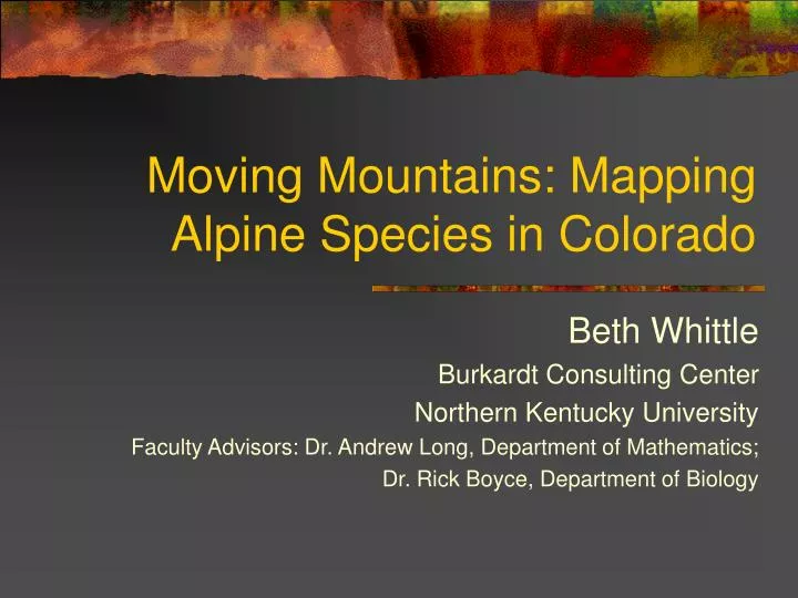
Moving Mountains: Mapping Alpine Species in Colorado. Beth Whittle Burkardt Consulting Center Northern Kentucky University Faculty Advisors: Dr. Andrew Long, Department of Mathematics; Dr. Rick Boyce, Department of Biology. Contents. Data Motivation/Goal

E N D
Moving Mountains: Mapping Alpine Species in Colorado Beth Whittle Burkardt Consulting Center Northern Kentucky University Faculty Advisors: Dr. Andrew Long, Department of Mathematics; Dr. Rick Boyce, Department of Biology
Contents • Data • Motivation/Goal • Presentation and Evaluation of Techniques • Current and Future Work
Presentation • Data
Data • There is collected data representing 63 sites. • For each site, the following information was collected: • Coordinates (UTM easting and northing) • Elevation • Aspect Value • Snow Depth • SICL • Presence and Absence Data for 78 plant species (1 if present; 0 if absent)
The green points represent the sampled sites. The distance between adjacent sites is approximately 50 meters.
Presentation • Data • Motivation/Goal
What do we want from this? • We want to predict the presence of species according to their location and environment. • Do we have the right data? • Do we have reasonable techniques?
Presentation • Data • Motivation/Goal • Techniques • 2 Dimensional • Variograms
Variogram Modeling • Data points are paired together • These pairs are separated into distance classes, and the mean sample variance among the members of each distance class is plotted. • Can we fit a model to this?
Example Shown on the left is a variogram for Eriogonum flavum Nutt. Var. xanthum (Small) Stokes (Yellow Buckwheat); on the right is the variogram with a spherical variogram model.
Presentation • Data • Motivation/Goal • Techniques • 2 Dimensional • Variography • Kriging
Kriging • Uses the variogram model in order to interpolate values. • Since we only have presence/absence data (z(xα)) for our species, our first thought is to interpolate a probability of presence. • Indicator Kriging
Example Here are our results from performing indicator kriging using the variogram model shown in the previous slide.
Presentation • Data • Motivation/Goal • Techniques • 2 Dimensional • Variography • Kriging • Complications
Complications • The data for Yellow Buckwheat generally follows our expectation of spatial autocorrelation: points close together should have a low variance, while points farther away should have a greater variance. • However, not all the species in this data set follow this paradigm.
Elevation: A Complicating Factor Look at site elevation; the problem is that members of the same distance class may have very similar elevations! Thus, if elevation is an important factor in determining presence/absence of species, then we would expect little variation amongst those sites at similar elevations.
Anisotropy • Perhaps the variogram cloud would be better fit by an anisotropic—where the degree of spatial autocorrelation is dependent on a directional component—model. • These are the results of a process called kernel smothing for Yellow Buckwheat. You can see that the contour lines are markedly elliptical, which suggests an anisotropic phenomenon.
Presentation • Data • Motivation/Goal • Techniques • 2-Dimensional • Variography • Kriging • Data Complications • Current and Future Work
Current Work • As evidenced by the earlier variogram, we think elevation is an important factor and thus would like to incorporate it into our variogram model. • 3-dimensional variography, where distance is defined in terms of UTM easting, UTM northing, and elevation. • We also see some anisotropy and thus want a model that reflects this.
Current Work • Fitting an anisotropic model to a 3-dimensional variogram cloud is really just a non-linear regression problem. • We need parameters for the rotation of the x, y, and z axes, as well as two scaling factors that characterize the ellipsoid that models the variogram cloud. • Thus, along with the sill, range, and nugget, that makes 8 parameters for our non-linear regression.
Current Work • We are working on a non-linear regression program, applied to our anisotropic, 3-dimensional variogram problem, in XLISP-STAT. • We would like to develop this program a bit more by including different model types, generalization to lower-dimension and isotropic cases, etc. • We hope to translate this into code for the R programming language.
Current and Future Work • Our next step is to use the 3-dimensional anisotropic variogram models in order to perform Kriging. • The grid that we need for the kriging is more complicated now; the grid is 3-dimensional because it now includes elevation. • A topographical map would be great right about now! But we will interpolate elevation for our purposes.
Some Preliminary Results:Allium geyeri S. Wats. (Geyer’s Onion) Kriging using a 2-dimensional, isotropic variogram model is on the left; Kriging using a 3-dimensional, anisotropic variogram model is on the right.
Some Preliminary Results: Artemsia scopulorum Gray (Alpine sagebrush) Recall the variogram model above; we cannot even fit a Gaussian variogram model to this, and thus Kriging gives the mean probability at all locations! Compare this to the 3-dimensional, anisotropic variogram.
Current and Future Work:Singular Value Decomposition • We use the Singular Value Decomposition to decompose the matrix of presence/absence data into UλVT, where U is a “factor” matrix, λ is the matrix of singular values, and VT is a matrix of “loadings.” • Do the factors exhibit spatial autocorrelation? • Under cursory examination, factors 1, 2, 3, and 5 do and the other factors do not. We can use these factors and their corresponding weights to reconstruct Kriging results for all of the species.
Reconstruction of Kriging Using Factors: Eriogonum flavum Nutt. var. xanthum (Small) Stokes. (Yellow Buckwheat)
References Boyce, R.L., R. Clark, and C. Dawson. 2005. Factors determining alpine species distribution on Goliath Peak, Front Range, Colorado, U.S.A. Arctic, Antarctic, and Alpine Research 37:89-90. Lay, David C. Linear Algebra and its Applications. 3rd ed. Boston: Addison-Wesley, 2003. Pebesma, Edzer J. et al. “The gstat Package.” March 21, 2006. <http://cran.r- project.org/doc/packages/gstat.pdf>. Pebesma, Edzer J. 2004. Multivariable geostatistcs in S: the gstat package. Computers and Geosciences, 30: 683-691. <http://plants.usda.gov>. The R Project for Statistical Computing. <http://www.r-project.org/>. Wackernagel, Hans. Multivariate Geostatistics: An Introduction with Applications. 2nd ed. Berlin: Springer, 1998. Weber, W.A. 1976. Rocky Mountain flora. Colorado Associated University Press, Boulder, Colorado. 479 p.
Thanks! If you have any comments, suggestions, etc, please send them to bcc@nku.edu. Burkardt Consulting Center: Dr. Mary Baggett and Patsy Sisson, Co-Directors; Catherine Smith, Yumi Muramatsu, Anthony DiBello, and Kelly Lay, Student Consultants Hans Wackernagel; Dr. Gail Mackin; Tim Meyers Funded by: Center for Integrative Natural Science and Mathematics (CINSAM); NKU Faculty Center for Teaching, Learning, and Technology.
Motivation for Kernel Smoothing • Perhaps the variogram cloud would be better fit by an anisotropic—where the degree of spatial autocorrelation is dependent on a directional component—model. • How can we visualize this when we have presence/absence data? • When we graph the variogram cloud in three space, we see the plane z=0 and z=1; not very helpful!
Kernel Smoothing • Using kernel smoothing, we literally “smooth” the 2 planes out into a surface that may reveal a trend. • We impose a grid on the data and, at each grid point, we use the surrounding data points in order to interpolate a value of presence.
Reconstruction of Kriging Using Factors: Mertensia lanceolata (Pursh) DC. (Prairie Bluebells)