Download
1 / 53
530 likes | 891 Views
Dormouse. Rabbit. Pika. Pig. Hippopotamus. Sheep. Cow. Alpaca. Blue whale. Fin whale. Sperm whale ... Dormouse. Cane-rat. Guinea pig. Mouse. Rat. Vole. Hedgehog. Gymnure ...

E N D
1. Phylogenetics I
2. Evolution
Evolution of new organisms is driven by Mutations The DNA sequence can be changed due to single base changes, deletion/insertion of DNA segments, etc. Selection bias
3. Theory of Evolution
Basic idea speciation events lead to creation of different species. Speciation caused by physical separation into groups where different genetic variants become dominant Any two species share a (possibly distant) common ancestor
4. The Tree of Life
Primate evolution A phylogeny is a tree that describes the sequence of speciation events that lead to the forming of a set of current day species; also called a phylogenetic tree.6. Morphological vs. Molecular
Classical phylogenetic analysis: morphological features: number of legs, lengths of legs, etc. Modern biological methods allow to use molecular features Gene sequences Protein sequences
Morphological topology Archonta Ungulata (Based on Mc Kenna and Bell, 1997) Rat QEPGGLVVPPTDA Rabbit QEPGGMVVPPTDA Gorilla QEPGGLVVPPTDA Cat REPGGLVVPPTEG From sequences to a phylogenetic tree There are many possible types of sequences to use (e.g. Mitochondrial vs Nuclear proteins). Mitochondrial topology (Based on Pupko et al.,) Nuclear topology (tree by Madsenl) (Based on Pupko et al. slide)11. Phylogenenetic trees
Leaves - current day species (or taxa � plural of taxon) Internal vertices - hypothetical common ancestors Edges length - �time� from one speciation to the next
12. Twists in molecular phylogenies
We have to emphasize that gene/protein sequence can be homologous for several different reasons: Orthologs -- sequences diverged after a speciation event Paralogs -- sequences diverged after a duplication event Xenologs -- sequences diverged after a horizontal transfer (e.g., by virus)
13. Paralogs
Consider evolutionary tree of three taxa: �and assume that at some point in the past a gene duplication event occurred. Gene Duplication
14. Paralogs
Speciation events Gene Duplication 1A 2A 3A 3B 2B 1B The gene evolution is described by this tree (A, B are the copies of the same gene).
15. Paralogs
Speciation events Gene Duplication 1A 2A 3A 3B 2B 1B If we happen to consider genes 1A, 2B, and 3A of species 1,2,3, we get a wrong tree that does not represent the phylogeny of the host species S S S
16. Types of Trees
A natural model to consider is that of rooted trees Common Ancestor
17. Types of trees
Unrooted tree represents the same phylogeny without the root node Depending on the model, data from current day species does not distinguish between different placements of the root.
Rooted versus unrooted trees a b c Tree c Represents the three rooted trees19. Total numbers of trees
For N taxa, Rooted bifurcating trees: (2n-3)!! = (2n-3)!/2n-2(n-2)! Unrooted bifurcating trees (2n-5)!! Tree shapes
20. Positioning Roots in Unrooted Trees
We can estimate the position of the root by introducing an outgroup: a set of species that are definitely distant from all the species of interest Aardvark Bison Chimp Dog Elephant Falcon Proposed root
21. Type of Data
Distance-based Input is a matrix of distances between species Can be fraction of residue they disagree on, or alignment score between them, or � Character-based Examine each character (e.g., residue) separately
22. Two methods of tree Construction
Distance- A weighted tree that realizes the distances between the objects. Parsimony � A tree with a total minimum number of character changes between nodes. We start with distance based methods, considering the following question: Given a set of species (leaves in a supposed tree), and distances between them � construct a phylogeny which best �fits� the distances.
23. Distance Matrix
Given n species, we can compute the n x n distance matrix Dij Dij may be defined as the edit distance between a gene in species i and species j, where the gene of interest is sequenced for all n species.
24. The distance between two sequences
Protein sequences: PAM BLOSUM DNA sequences Jukes-Cantor HGY Kimura 2-Parameter
25. General Stationary Time-reversible Model
R = Time reversibility: pirij = pjrji (Diagonal elements such that rows sum to zero)
26. General Stationary Time-reversible Model
P(t) = eRt Given rates, one can find transition probabilities, and vice-versa.
27. Jukes-Cantor
R =
28. Jukes-Cantor
P(no mutation) = e-4/3ut P(at least one mutation) = 1-e-4/3ut Ds = � * (1-e-4/3ut) D ? ut = -3/4 ln (1-4/3 * Ds)
29. Kimura 2-Parameter
R = a/b = transition/transversion bias ? R a+2b = 1 per unit time A C G T
30. Kimura 2-Parameter
a=R/(R+1), b=0.5/(R+1)
31. HKY (Hasegawa, Kishino, Yano)
R = k = transversion / transition Some rules of thumb: Use simpler models with shorter sequences (< 200 bp). Otherwise, use a model as complex as necessary. Compare results from more than one method. Some rules of thumb: Use simpler models with shorter sequences (< 200 bp). Otherwise, use a model as complex as necessary. Compare results from more than one method.
32. Distances in Trees
Edges may have weights reflecting: Number of mutations on evolutionary path from one species to another Time estimate for evolution of one species into another In a tree T, we often compute dij(T) - the length of a path between leaves i and j
33. Distance in Trees: an Exampe
d1,4 = 12 + 13 + 14 + 17 + 12 = 68
34. Fitting Distance Matrix
Given n species, we can compute the n x n distance matrix Dij Evolution of these genes is described by a tree that we don�t know. We need an algorithm to construct a tree that best fits the distance matrix Dij
35. Reconstructing a 3 Leaved Tree
Tree reconstruction for any 3x3 matrix is straightforward We have 3 leaves i, j, k and a center vertex c Observe: dic + djc = Dij dic + dkc = Dik djc + dkc = Djk
36. Reconstructing a 3 Leaved Tree
37. Trees with > 3 Leaves
An tree with n leaves has 2n-3 edges This means fitting a given tree to a distance matrix D requires solving a system of �n choose 2� equations with 2n-3 variables This is not always possible to solve for n > 3
38. Additive Distance Matrices
Matrix D is ADDITIVE if there exists a tree T with dij(T) = Dij NON-ADDITIVE otherwise
39. Distance Based Phylogeny Problem
Goal: Reconstruct an evolutionary tree from a distance matrix Input: n x n distance matrix Dij Output: weighted tree T with n leaves fitting D If D is additive, this problem has a solution and there is a simple algorithm to solve it
40. Using Neighboring Leaves to Construct the Tree
Find neighboring leaves i and j with parent k Remove the rows and columns of i and j Add a new row and column corresponding to k, where the distance from k to any other leaf m can be computed as: Dkm = (Dim + Djm � Dij)/2 Compress i and j into k, iterate algorithm for rest of tree
41. Finding Neighboring Leaves
To find neighboring leaves we simply select a pair of closest leaves.
42. Finding Neighboring Leaves
To find neighboring leaves we simply select a pair of closest leaves. WRONG
43. Finding Neighboring Leaves
Closest leaves aren�t necessarily neighbors i and j are neighbors, but (dij = 13) > (djk = 12) Finding a pair of neighboring leaves is a nontrivial problem!
44. Neighbor Joining Algorithm
In 1987 Naruya Saitou and Masatoshi Nei developed a neighbor joining algorithm for phylogenetic tree reconstruction Finds a pair of leaves that are close to each other but far from other leaves: implicitly finds a pair of neighboring leaves Advantages: works well for additive and other non-additive matrices, it does not have the flawed molecular clock assumption
45. Constructing additive trees: The neighbor joining algorithm
Let i, j be neighboring leaves in a tree, let k be their parent, and let m be any other vertex. The formula shows that we can compute the distances of k to all other leaves. This suggest the following method to construct tree from a distance matrix: Find neighboring leaves i,j in the tree, Replace i,j by their parent k and recursively construct a tree T for the smaller set. Add i,j as children of k in T.
46. Neighbor Finding
How can we find from distances alone a pair of nodes which are neighboring leaves? Closest nodes aren�t necessarily neighboring leaves. Next we show one way to find neighbors from distances.
47. Neighbor Finding: Seitou & Nei algorithm
Theorem (Saitou & Nei) Assume all edge weights are positive. If D(i,j) is minimal (among all pairs of leaves), then i and j are neighboring leaves in the tree. Definitions
48. Naive Implementation: Initialization: ?(L2) to compute d(r,i) and C(i,j) for all i,j?L. Each Iteration: O(L2) to find the maximal C(i,j). O(L) to compute {C(m,k):m? L} for the new node k. Total of O(L3).
Complexity of Neighbor Joining Algorithm m k r C(m,k)
49. Complexity of Neighbor Joining Algorithm
Using Heap to store the C(i,j)�s: Input: Distance matrix D= d(i,j), and an arbitrary object r. Initialization: ?(L2) to compute and heapify the C(i,j)�s in a heap H. Each Iteration: O(log L) to find and delete the maximal C(i,j) from H. O(L) to add the values {d(k,m)} to D, for all objects m. O(L) to delete {d(m,i), d(m,j)} from D (for all m). O(L log L) to delete {C(i,m), C(j,m)} and add C(k,m) from H, for all objects m. Total of O(L2 log L). (implementation details are omitted)
50. Neighbor Joining Algorithm
Applicable to matrices which are not additive Known to work good in practice The algorithm and its variants are the most widely used distance-based algorithms today.
51. The Four Point Condition
Compute: 1. Dij + Dkl, 2. Dik + Djl, 3. Dil + Djk 1 2 3 2 and 3 represent the same number: the length of all edges + the middle edge (it is counted twice) 1 represents a smaller number: the length of all edges � the middle edge
52. The Four Point Condition: Theorem
The four point condition for the quartet i,j,k,l is satisfied if two of these sums are the same, with the third sum smaller than these first two Theorem : An n x n matrix D is additive if and only if the four point condition holds for every quartet 1 = i,j,k,l = n
53. Least Squares Distance Phylogeny Problem
If the distance matrix D is NOT additive, then we look for a tree T that approximates D the best: Squared Error : ?i,j (dij(T) � Dij)2 Squared Error is a measure of the quality of the fit between distance matrix and the tree: we want to minimize it. Least Squares Distance Phylogeny Problem: finding the best approximation tree T for a non-additive matrix D (NP-hard).