Download
1 / 35
350 likes | 542 Views
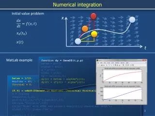
Electrostatics numerical integration. Electrostatics. +Q. +Q. +Q. - Q. electric field. r. y. r. y. . x. x. . . symmetry. r. y. . x. . . z. r. y. x. Gauss's law. infinite charged sheet. Voltage -- work. Voltage – work Superposition. numerical integration. y.

E N D
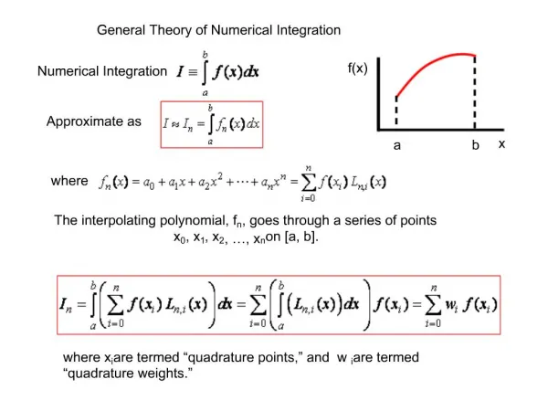
Electrostatics numerical integration
Electrostatics +Q +Q +Q - Q
r y r y x x symmetry
r y x
z r y x Gauss's law
Voltage – work Superposition
y b x + Dz z a
y b x + Dz z a
j = 3 y b j = 2 x j = 1 Rj,k k = 1 + k = 2 Dz z k = 3 a
j 1 2 3 n-1 n 1 2 3 b k m-1 m a
j = 3 y b j = 2 x j = 1 Rj,k k = 1 + k = 2 Dz z k = 3 a
y b x + z a
5 13 6 8 4 3 12
y b x + z a
y b x A + dz z a
clear; clf n=3; a=12; m=3; b=16; dz=12; V=0; for j=1: n-1 for k=1: m-1 A=[dz ((n/2)-j)*(a/(n-1)) ((m/2)-k)*(b/(m-1))]; R=norm(A); V=V+1/R; end end V V = .3077 = 4/13
plot the result of the previous calculation
clear n=3; a=12; m=3; b=16; dz=12; V=0; for j=1: n-1 for k=1: m-1 A=[dz ((n/2)-j)*(a/(n-1)) ((m/2)-k)*(b/(m-1))]; R=norm(A); V=V+1/R; end end V V = .3077 = 4/13 #1
for w=-1:2 for ddz=1:10; dz=ddz*10^w; V=0; loglog(dz,V,'o') hold on end end xlabel('dz','fontsize',18) ylabel('V','fontsize',18) set(gca,'fontsize',18) whitebg('black') #1
clear n=3; a=12; m=3; b=16; dz=12; V=0; for j=1: n-1 for k=1: m-1 A=[dz ((n/2)-j)*(a/(n-1)) ((m/2)-k)*(b/(m-1))]; R=norm(A); V=V+1/R; end end V V = .3077 = 4/13 #1 #2 ;
for w=-1:2 for ddz=1:10; dz=ddz*10^w; V=0; loglog(dz,V,'o') hold on end end xlabel('dz','fontsize',18) ylabel('V','fontsize',18) set(gca,'fontsize',18) whitebg('black') #1 #2
for w=-1:2 for ddz=1:10; dz=ddz*10^w; V=0; loglog(dz,V,'o') hold on end end xlabel('dz','fontsize',18) ylabel('V','fontsize',18) set(gca,'fontsize',18) whitebg('black')
Electric field normal to a surface • Two regions – • The first region is very close to the surface so the surface almost appears to be infinite in extent. • The second is at distances that are large with respect to the dimensions of the surface and the surface appears to be a point charge.
quadrature function ”quad” • the function “quad” approximates the integral of a function from a to b with an error of 10- 6 using “recursive adaptive Simpson quadrature.” • This also holds true for “dblquad” & “triplequad.”
% electric field at different distances clear;clf for z= 1: 100 f=inline('10*z./(sqrt(x.^2+y.^2+(z/10).^2).^3)'); coefficient(z) =dblquad(f, -.5, .5, -.5, .5, [ ],'',z); end loglog(1: 100, coefficient,'-s') hold on plot([10/(10^(1/2)) 100], [1000 1],'--','linewidth', 3) xlabel ('z/a','fontsize', 18) ylabel ('coefficient','fontsize', 18) set(gca,'fontsize', 18) grid on legend ('numerical integration','slope = -2', 3)
12 y V(z = 6) = ? Find V(z) 12 12 x 6 z
6 6 12 y V(z = 6) = ? Find V(z) 6 x z