Download
1 / 53
540 likes | 731 Views
Statistical data analysis in functional genomics. Wolfgang Huber Genome Biology Unit EMBL Predoc Course 2009. Download dataset E-MEXP-1422 (e.g. using Bioconductor). Go to ArrayExpress website. Microarray Experiment. si-GFP. Si-PROX1 (#1). Si-PROX1 (#2). colon cancer cell line.

E N D
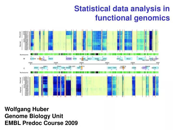
Statistical data analysis in functional genomics Wolfgang Huber Genome Biology Unit EMBL Predoc Course 2009
Download dataset E-MEXP-1422 (e.g. using Bioconductor) Go to ArrayExpress website
Microarray Experiment si-GFP Si-PROX1 (#1) Si-PROX1 (#2) colon cancer cell line
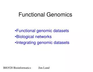
samples: mRNA from tissue biopsies, cell lines fluorescent detection of the amount of sample-probe binding arrays: probes = gene-specific DNA strands tissue A tissue B tissue C ErbB2 0.02 1.12 2.12 VIM 1.1 5.8 1.8 ALDH4 2.2 0.6 1.0 CASP4 0.01 0.72 0.12 LAMA4 1.32 1.67 0.67 MCAM 4.2 2.93 3.31 marray data
Outliers: data points whose distance from the box is larger than 1.5 times the interquartile range. The whiskers extend to the last point which is not an outlier. A boxplot is a graphical representation of the Five-number summary: minimum, 1st quartile, median, 3rd quartile, maximum Boxplot 50% of the data is in the box “Interquartile range” Whisker Outliers Outlier Median 50% of the data is above 50% of the data is below 25% of the data is below the box 25% of the data is above the box
Regression Slope: Different amount of extracted RNA Different labeling efficiency Baseline: Different background fluorescence
A complex measurement process lies between RNA concentrations and intensities The problem is less that these steps are ‘not perfect’; it is that they vary from array to array, experiment to experiment.
spike-in data log2 Cope et al. Bioinformatics 2003
Should really be called calibration; has nothing to do with the normal distribution Four major approaches: Linear scaling: x → ax Affine (e.g. vsn): x → ax + b Monotone smooth (e.g. loess): x → f(x) Rank (e.g. quantile normalisation): x → rank(x) Normalisation
Statistics 101 biasaccuracy precision variance
Basic dogma of data analysis Can always increase sensitivity on the cost of specificity, or vice versa, the art is to - optimize both, then - find the best trade-off. X X X X X X X X X
Hypothesis testing Two hypotheses in competition: • H0: the null hypothesis, usually the more conservative, more specific, better understood • H1 or HA: alternative hypothesis, often corresponds to the statement that we want to demonstrate Examples of null hypotheses: • The coin is fair • The new drug is no better (or worse) than a placebo • There is no difference in weight between two groups of mice
Karl Popper (1902-1994) Logical asymmetry between verification and falsifiability No number of positive outcomes at the level of experimental testing can confirm a scientific theory, but a single counterexample is logically decisive: it shows the theory is false Neyman-Pearson theory of hypothesis testing (~1950): goal is to use the data to reject H0 (with high confidence) - which implies the complement of H0.
Hypothesis testing We need something to measure how far an observation is from what we expect to see if H0 is correct: a test statistic Example: number of heads obtained when tossing a coin a given number of times. We expect that this number should be close to half the number of tosses. But what is „close“? We can use combinatorics / probability theory to quantify this. For example, in 12 tosses, the probability of seeing exactly 8 heads is
Significance level The p-value is the probability that the test statistic is as or more extreme than the observed value. Practitioners like tests where this probability can be explicitly computed through a mathematical formula (t-test, Wilcoxon, hypergeometric…). If not, one can often still estimate it by random permutation or bootstrapping Historically, some people agreed that for many instances, a significance level α =0.05 was a useful cutoff. But there is nothing magic about this number. Two views: Strength of evidence for a certain (negative) statement Rational decision support
Binomial distribution How is the test statistic distributed if H0 is correct ? P(Heads <= 1) = 0.01074 P(Heads >= 9) = 0.01074
One-sided vs two-sided tests If HA is “the coin is biased”, we do not specify the direction of the bias and must be ready for both alternatives (many heads or many tails) This is a two-sided test. If the total level of the test α is e.g. 0.05, we allow α/2 for bias towards tail and α/2 for bias towards head. If HA is “the coin is biased towards heads”, we specify the direction of the bias and the test is one-sided. One-sided test is more powerful – but it depends on a greater amount of prior information
Errors in hypothesis testing Decision Truth
One sample t-test t-statistic (1908, William Sealy Gosset, pen-name “Student”) n is the number of observations Without n: z-score, a relative measure of distance With n: t-statistic. Its null distribution can be computed: t-distribution with a parameter that is called “degrees of freedom” equal to n-1
t-test If H0 is correct, t follows a known distribution: t-distribution The shape of the t-distribution depends on the number of observations: if the average is made of n observations, if follows the t-distribution with n-1 degrees of freedom (tn-1). If n is large, tn-1 is close to a normal distribution If n is small, tn-1 is more spread out than a normal distribution (penalty because we had to estimate the standard deviation using the data).
One sample t-test: example Consider the following 10 data points: -0.01, 0.65, -0.17, 1.77, 0.76, -0.16, 0.88, 1.09, 0.96, 0.25 We are wondering if these values come from a distribution with a true mean of 0. H0: the true mean is 0; HA: the true mean is not 0 These 10 data points have a mean of 0.60 and a standard deviation of 0.62. From these numbers, we can calculate the t-statistic: t = 0.60 / 0.62 * 101/2 = 3.0
t9 2.5% 2.5% -2.26 2.26 One sample t-test: example Since we have 10 observations, we must compare our observed t-statistic to the t distribution with 9 degrees of freedom Since t = 3.01 > 2.26, the difference is significant at the 5% level. Exact p-value: P( |t| >= 3.01) = 0.014
5% 2.5% 2.5% One-sided vs two-sided test One-sided e.g. HA: μ>0 Two-sided e.g. HA: μ=0
Two samples t-test Do two different samples have the same mean ? Test-statistic: Where y and x are the average of the observations in both populations SE is the standard error for the difference (see a book for details) If H0 is correct (no difference in mean), the test statistics follows a t distribution with n+m-2 degrees of freedom (n, m the number of observations in each sample).
Comments and pitfalls The derivation of the t-distribution assumes that the observations are independent and that they follow a normal distribution. If the data are not normal (e.g. heavier tails), that is actually rarely a problem for the t-test. If the data are dependent, then p-values will likely be totally wrong (e.g., for positive correlation, too optimistic).
Multiple testing • Classical hypothesis test: • null hypothesis H0, alternative H1 • test statistic X t(X) • a = P( t(X) Grej | H0) type I error (false positive) • b = P( t(X) Grej | H1) type II error (false negative) • When n tests are performed, what is the extent of type I errors, and how can it be controlled? • E.g.: 20,000 tests at a=0.05, all with H0 true: expect 1,000 false positives
p-values: a mixture null alternative Slide37
Experiment-wide type I error rates Family-wise error rate: P(V > 0), the probability of one or more false positives. For large m0, this is difficult to keep small. False discovery rate: E[ V / max{R,1} ], the expected fraction of false positives among all discoveries. Slide38
Benjamini Hochberg multiple testing adjustmentcontrol siRNA vs PROX1 siRNA #1 slope: alpha / #genes
Benjamini Hochberg multiple testing adjustmentcontrol siRNA vs PROX1 siRNA #1 rawp Bonferroni BH [1,] 9.67e-06 0.215 0.215 [2,] 2.94e-05 0.655 0.242 [3,] 3.25e-05 0.725 0.242 [4,] 7.28e-05 1.000 0.261 [5,] 8.01e-05 1.000 0.261 [6,] 8.90e-05 1.000 0.261
Independent filtering From the set of 22,000 probes, first filter out those that seem to report negligible signal (say, 40%), then formally test for differential expression on the rest. Conditions under which we expect negligible signal : Target gene is absent, or just weakly expressed, in both samples. (Probes will still report noise and cross-hybridization.) Probe fails to detect the target. Slide45
Increased detection rates Stage 1 filter: compute variance, across samples, for each probeset, and remove the fraction θ that are smallest Stage 2: standard two-sample t-test ALL data
Increased detection rate implies increased power only if we are still controlling type I errors at the nominal level. Increased power? • Concerns: • Have we thrown away good genes? • Use a data-driven criterion in stage 1, but do type I error consideration only on number of genes in stage 2 • Informal justification: • Filter does not use covariate information ALL data Slide47
Marginal control: independence of stage 1 and stage 2 statistics under the null hypothesis For genes for which the null hypothesis is true (X1 ,..., Xn exchangeable), f and g are statistically independent in both of the following cases: • Normally distributed data: f (stage 1): overall variance (or mean) g (stage 2): the standard two-sample t-statistic, or any test statistic which is scale and location invariant. • Non-parametrically: f: any function that does not depend on the order of the arguments. E.g. overall variance, IQR. g: the Wilcoxon rank sum test statistic. Both can be extended to the multi-class context: ANOVA and Kruskal-Wallis. Slide48
Diagnostics odds ratio = 4.4 abs. value of t-statistic (stage 2) ALL data overall standard deviation (stage 1)