Download
1 / 10
280 likes | 1.32k Views
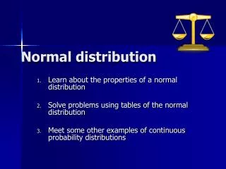
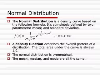
NORMAL DISTRIBUTION. Normal distribution- continuous distribution. Normal density: bell shaped, unimodal- single peak at the center, symmetric. Completely described by its center of symmetry - mean μ and spread - standard deviation σ. μ.

E N D
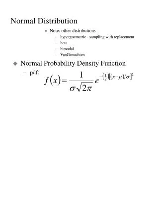
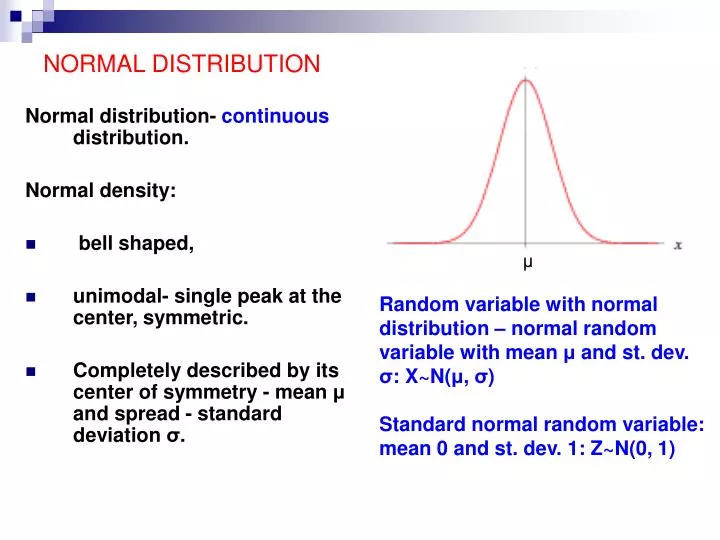
NORMAL DISTRIBUTION Normal distribution- continuous distribution. Normal density: • bell shaped, • unimodal- single peak at the center, symmetric. • Completely described by its center of symmetry - mean μand spread - standard deviation σ. μ Random variable with normal distribution – normal random variable with mean μ and st. dev. σ: X~N(μ, σ) Standard normal random variable: mean 0 and st. dev. 1: Z~N(0, 1)
NORMAL DISTRIBUTION-CHANGING LOCATION AND SCALE CHANGING SCALE σ CHANGING LOCATION μ μ1 μ2 “peaky” density “flatter” density 1=σ1 < σ2 = 2 0=μ1 < μ2 =1 Changes in mean/location cause shifts in the density curve along the x-axis. Changes in spread/standard deviation cause changes in the shape of the density curve.
Why Bother with Normal Distributions? • Normal distributions are great descriptions-models-approximations for many data sets such as weights, heights, exam scores, experimental errors, etc. • Great descriptions of results-outcomes of many chance driven experiments. • Statistical inference based on normal distribution works well for many (approximately) symmetric distributions. • HOWEVER, remember that not everything or everybody is normal!
THE EMPIRICAL RULE - THE 68-95-99.7 RULE Areas under the normal curve are probabilities (as under any density curve). Special areas under the normal density curve: • Approximately 68% of the observations fall within 1 standard deviation of the mean • Approximately 95% of the observations fall within 2 standard deviations of the mean • Approximately 99.7% of the observations fall within 3 standard deviations of the mean
THE EMPIRICAL RULE - contd The range "within one/two/three standard deviation(s) of the mean" is highlighted in green. The area under the curve over this range is the rel. frequency of observations in the range. That is, 0.68/95/99.7 = 68%/95%/99.7% of the observations fall within one/two/three standard deviation(s) of the mean, or, 68%/95%/99.7% of the observations are between (μ – 1/2/3σ) and (μ + 1/2/3σ).
AREAS UNDER THE NORMAL CURVE Normal probabilities = areas under the normal curve are tabulated for the standard normal distribution (front cover of your text book). In looking for probabilities keep in mind: Symmetry of the normal curve and P(Z=a)=0 for any a. FIND: P(Z < 0.01) = 0.504 P(Z ≤ -0.01 ) = 0.496 P(Z < 0) = 0.5 P( Z < 2.92)= 0.9982 P(Z>2.92)=1-0.9982=0.0018 or, by symmetry =P(Z< - 2.92)=0.0018 P(-1.32< Z <1.2)=0.8849 – 0.0934=0.7915 SUMMARY OF RULES we used above: P(Z>a)=1-P(Z< -a) P(a < Z < b) = P(Z < b)- P( Z < a)
GENERAL NORMAL DISTRIBUTION IF X~N(μ, σ) then Z = ~N(0, 1) standard normal. standardization Example. Suppose that the weight of people in NV follows normal distribution with mean 150 and standard deviation 20 lb. Find the probability that a randomly selected Nevadan weighs at most 160 lb; b) over 160 lb. Solution. Let X= weight of a randomly selected Nevadan. X~N(150, 20). • P(X ≤ 160) = • P(X>160)= 1 - P(X ≤ 160) =1 – 0.6915 = 0.3085.
NORMAL PERCENTILES Given that P(Z < p)=0.95 find p. Here p is called 95thpercentile of Z. Inside the table I looked for 0.95. Found 0.9495 and 0.9505. Used z-value corresponding to the midpoint (0.95) between the two available probabilities 1.645. p=1.645 If an available probability is closer to the one we need, use the z-value corresponding to that probability. 0.95 p=?
NORMAL PERCENTILES, CONTD. EXAMPLE. Suppose scores X on a test follow a normal distribution with mean 430 and standard deviation 100. Find 90th percentile of the scores, that is find score x such that P(X ≤ x)=0.9. Solution. Since we start with a normal but NOT STANDARD normal distribution, we have to standardize at some point: 0.9 = P(X ≤ x) = get equation: x - 430 =128 x = 558 90% of students scored 558 or less. 0.90 z =1.28
EXAMPLE Height of women follows normal distribution with mean 64.5 and standard deviation of 2.5 inches. Find a) The probability that a woman is shorter than 70 in. b) The probability that a woman is between 60 and 70 in tall. c) What is the height 10% of women are shorter than, i.e. what is the 10th percentile of women heights? SOLUTION. X= women height; X~N(64.5, 2.5). a) P(X <70)=P(Z< (70-64.5)/2.5)=P(Z<2.2)=0.9861 b) P( 60 < X < 70) = P( (60-64.5)/2.5) < Z < (70-64.5)/2.5)=P(-1.8< Z < 2.2)= P( Z <-2.2) – P( Z < -1.8) = 0.9861 – 0.0359 = 0.9502. c) 10th percentile of X =? 0.1=P( X< x) = P( Z< (x-65.5)/2.5), so -2.33=(x-65.5)/2.5; x=59.675. 10% of women are shorter than 59.675 in.