Download
1 / 17
180 likes | 380 Views
The H 2 O molecule: converging the size of the simulation box . Objectives - study the convergence of the properties with the size of the unit cell. H 2 O molecule: example of a very simple input file.

E N D
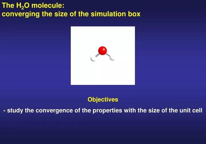
The H2O molecule: converging the size of the simulation box Objectives - study the convergence of the properties with the size of the unit cell
H2O molecule: example of a very simple input file Go to the directory where the exercise of the H2O molecule is included Inspect the input file, h2o.fdf Examine in detail the different input variables, more information at http://www.icmab.es/siesta and follow the link Documentations, Manual Number of different species and atoms present in the unit cell List of different species Position of the atoms Example of a first-principles simulation: no input from experiment
Many variables will take the default value PAO.BasisSize (Basis set quality) DZP XC.Functional (Exchange and correlation functional) LDA XC.Authors (Flavour of the exchange and correlation) CA SpinPolarized (Are we performing an spin polarized calc.) .false. … and many others. For a detailed list, see fdf.log after running the code.
H2O molecule with Periodic Boundary Conditions (PBC) Strategy: the supercell approach Introduce a vacuum region that should be large enough that periodic images corresponding to adjacent replicas of the supercell do not interact significantly. Although our system is aperiodic (a molecule), Siesta still does use PBC Make sure that the required physical and chemical properties are converged with the size of the supercell
H2O molecule with Periodic Boundary Conditions (PBC) The default unit cell The lattice vectors will be diagonal, and their size will be the minimum size to include the system without overlap with neighboring cells, plus a buffer layer (10%)
H2O molecule: the first run of Siesta (we are doing better, 0.003 thousand of atoms) Run the code, siesta < h2o.fdf > h2o.default.out The name of the output file is free, but since we are running the H2O molecule with the default unit cell, this seems very sensible… Check that you have all the required files A pseudopotential file (.vps or .psf) for every atomic specie included in the input file For H and O within LDA, you can download it from the Siesta web page. Wait for a few seconds… and then you should have an output
H2O molecule with Periodic Boundary Conditions (PBC) For molecules, Let’s make a tour on the different output files: Inspect the output file, h2o.default.out How many SCF cycles were required to arrive to the convergence criterion? How much is the total energy of the system after SCF? How large is the unit cell automatically generated by Siesta? How much is the electric dipole of the molecule (in electrons bohr)?
H2O molecule: convergence with the size of the supercell Modify the input file, introducing explicitly the supercell Define the supercell here Run the code, changing the lattice constant from 8.00 Å to 15.00 Å in steps of 1.0 Å. Save each input file in a separate file. siesta < h2o.fdf > h2o.your_lattice_constant.out
H2O molecule: convergence with the size of the supercell Tabulate the total energy as a function of the lattice constant grep “Total =” h2o.*.out > h2o.latcon.dat Edit the h2.latcon.dat file, and leave only two columns Lattice constant (Å) Total energy (eV) These numbers have been obtained with siesta-3.0-b, compiled with the g95 compiler and double precision in the grid. Numbers might change slightly depending on the platform, compiler and compilation flags
H2O molecule: convergence with the size of the supercell Plot the total energy versus the lattice constant gnuplot plot “h2o.latcon.dat” using 1:2 with lines
H2O molecule: the most important point: Analyze the results Ideally, for a molecule any property should be independent of the size of the simulation box… …but this is not the case (at least for the energy) in the case of H2O. Why? Water molecule has a dipole
H2O molecule: the most important point, analyze the results puntual dipole located at unit vector along puntual dipole located at When calculating the energy of an aperiodic system using periodic boundary conditions, one is interested only in the energy, E0 in the limit L , where L is the linear dimension of the supercell. The energy calculated for a finite supercell E(L) differs from E0, because of the spurious interactions of the aperiodic charge density with its images in neighboring cells To estimate E0 from the calculatedE(L), we need to know the asymptotic behaviour of the energy on L Water molecule has a dipole The electrostatic interaction between dipoles decay as L-3, with L the separation between dipoles G. Makov and M. C. Payne, Phys. Rev. B 51, 4014 (1995)
H2O molecule: the most important point, analyze the results To estimate E0 from the calculatedE(L), we need to know the asymptotic behaviour of the energy on L But this dependence is not enough. Furthermore, these interactions induce changes in the aperiodic charge density itself, which depends on L In other words, the dipole also depends on L If the molecule has a permanent dipole, then the induced dipole will beO(L-3) because the field generated by a dipole decays as L-3 G. Makov and M. C. Payne, Phys. Rev. B 51, 4014 (1995)
H2O molecule: convergence of the dipole moment grep “Electric dipole (a.u.)” h2o.*.out > h2o.dipole.dat Edit h2o.dipole.dat and leave only the lattice constant and the components of the dipole moment (with the particular orientation of our molecule, only the y component does not vanish). gnuplot plot “h2o.dipole.dat” using 1:3 with lines Lattice constant (Å) Electric dipole (a.u.)
H2O molecule: convergence of the dipole moment , and fitting parameters If the molecule has a permanent dipole, then the induced dipole will beO(L-3) because the field generated by a dipole decays as L-3
H2O molecule: the most important point, analyze the results , , and fitting parameters To estimate E0 from the calculatedE(L), we need to know the asymptotic behaviour of the energy on L If we replace p by p(L), then the leading contribution to the electrostatic energy reflecting the (dipole-induced)-dipole interaction is of the order ofO(L-6) Direct dipole-dipole interaction (Dipole-induced) - dipole interaction G. Makov and M. C. Payne, Phys. Rev. B 51, 4014 (1995)
H2O molecule: the most important point, analyze the results , , and fitting parameters To estimate E0 from the calculatedE(L), we need to know the asymptotic behaviour of the energy on L If we replace p by p(L), then the leading contribution to the electrostatic energy reflecting the (dipole-induced)-dipole interaction is of the order ofO(L-6) Direct dipole-dipole interaction (Dipole-induced) - dipole interaction G. Makov and M. C. Payne, Phys. Rev. B 51, 4014 (1995) E0 is the energy we are interested in