Download
1 / 34
340 likes | 519 Views
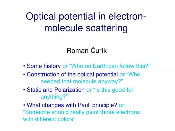
Optical potential in electron-molecule scattering. Some history or “Who on Earth can follow this?” Construction of the optical potential or “Who needed that molecule anyway?” Static and Polarization or “Is this good for anything?”

E N D
Optical potential in electron-molecule scattering • Some history or “Who on Earth can follow this?” • Construction of the optical potential or “Who needed that molecule anyway?” • Static and Polarization or “Is this good for anything?” • What changes with Pauli principle? or “Someone should really paint those electrons with different colors” Roman Čurík
History • 1956 – W.B.Riesenfeld and K.M. Watson summarized Perturbation expansions for energy of many-particle systems. Different choices of O leads to different perturbation methods: - Brillouin-Wigner- Rayleigh-Schrödinger- Tanaka-Fukuda- Feenberg
1958 – M.H. Mittleman and K.M. Watson applied Feenberg perturbation method for electron-atom scattering with exchange effects neglected • 1958 – Feshbach method • 1959 – B.A. Lippmann, M.H.Mittleman and K.M. Watson included Pauli’s exclusion principle into electron-atom scattering formalism • 197X – C.J.Joachain and simplified Feenberg method without exchange
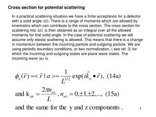
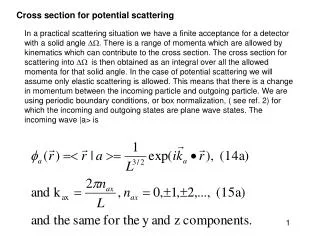
N+1 electron scattering • Formulation in CMS • Nuclear mass >> mass of electrons • Vibrations and rotations of molecule not considered • Electronically elastic scattering N electrons M nuclei rN r r2 scattered electron r1 molecule
Total hamiltonian H is split into free part H0and a “perturbation” V:
Exact solution can be provided by N+1 electron Lippmann-Schwinger equation Function describes both the elastic and inelastic scattering. For example it can be expanded in diabatic expansion over states of the target as:
Since we don’t have any rearrangement and target remains in the same electronic state, can we reduce the size of the problem and formulate scattering equations as for scattering of a single electron by some single-electron optical potential? where corresponds to the elastic (coherent) part of the total wave function .
We define projection operator onto ground states: Elastic part can be obtained by projection Full N+1 L-S equations for are
By applying from the left we get where the elastic part of the T operator can be defined as follows,
We have projected L-S equation Definition of optical potential gives desired form or
Thus the optical potential Voptis defined as an operator which, through the Lippmann-Schwinger equation leads to the exact transition matrix TC corresponding to the elastic scattering of the incident particle by the molecule. Finally we project above equation onto the ground state of molecule via and the single-electron equation is obtained:
Where is a single-particle optical potential obtained by The definition of Vopt does not imply that optical potential is an Hermitian operator. In fact, hermitian Voptwould lead to TC such that is unitary. In fact after applying of machinery of optical theorem it can be shown that
Optical potential and the many-body problem Following the method of Watson et al we introduce an operator F such that Thus, in contrast with Π0, the new operator F reconstructs the full many-body wave function from its elastic scattering part. In order to connect it with many-body problem we start from the full N+1 electron L-S equation:
and apply Π0 from left thus the optical potential , which does not act on the internal coordinates of the target, is given by
In order to determine we must therefore find the operator F. To carry out this we just play with above equations with extracted from above we get
or finally This is an exact L-S equation for F, which can be solved in few ways: • 2 body scattering matrices lead to Watson equations • Perturbation Born series in powers of the interaction V, namely Once again, single particle optical potential was
Optical potential for the molecules First order term leads in so-called Static-Exchange Approximation with exchange part still missing because Pauli exclusion effects have been neglected so far with
HF approximation Let’s take first term:
Thus the first order optical potential provides the static (and exchange) potential generated by nuclei and fixed bound state wave function of the molecule: with HF density
How good is Static (-Exchange) Approximation? • Static (-Exchange) approximation leads to correct interaction at very small distances from nuclei. • Therefore one can expect results improving with higher collision energies ( > 10 eV) and for largerscattering angles that are ruled by electrons withsmall impact parameters. • is Hermitian and therefore no electronically inelastic processes can be described by this term.
(Correlation -) Polarization We notice that where n runs over all intermediate states of the target except the ground state. Then
Adiabatic approximation assumes that the change of kinetic energy may be neglected comparing to excitation energies wn-w0, then Adiabatic approximation is local (non-local properties have been removed with kinetic energy operator neglected in denominator) and real. So again does not account for the removal of particles from elastic channel above excitation threshold.
Angular expansion of the Coulomb operator gives approximate expression
The adiabatic approximation to second order optical potential then becomes where is the dipole polarizability of the molecule. Thus we see if the orbital relaxation caused by strongest second order of interaction V is allowed, rise of a long-range potential behaved as r-4 can be noticed.
Approximation of the average excitation energy Introducing complete set of plane waves we obtain:
The effect of Pauli principle We define asymptotic states of l-th electron being in continuum as (0-th coordinate stands for scattered particle now) Our scattering problem can be defined via solutions of full N+1 electron Schrödinger equation where is antisymmetric in all pairs of electrons.
A boundary condition must be added to fix uniquely. The physics of the problem dictates the boundary condition: As rl approaches infinity, for l arbitrary, approaches the asymptotic form For evaluation of cross section we need to calculate the flux of the scattered electrons “0” only.
That is, all the N+1 particles enter the problem symmetrically. Each of them at infinity carries the same ingoing and the same outgoing flux. Hence the total flux is N+1 times the flux of one particle. Since only the out/in ration of fluxes appear in cross section it is sufficient to calculate the flux of particle 0 alone. Or, we may regard particle 0 as distinguishable in obtaining scattering cross section from . The flux of “0” electrons scattered is calculated from
Final expressions for the optical potential for undistinguishable particles have very similar form This time V is modified interaction potential: where swaps 0-th and i-th electrons. Thus the additional exchange term has in coordinate representation form (HF orbitals assumed):
Exchange part is non-local and short-range interaction as can be seen from its effect on wave function Second order using HF approximation leads to the sum of 2 terms, called polarization and correlation contributions as follows:
V(1) 0 excitations (only ground state) • V(2) single excitations • V(3) double excitations • V(N) …..