Download
1 / 26
260 likes | 383 Views
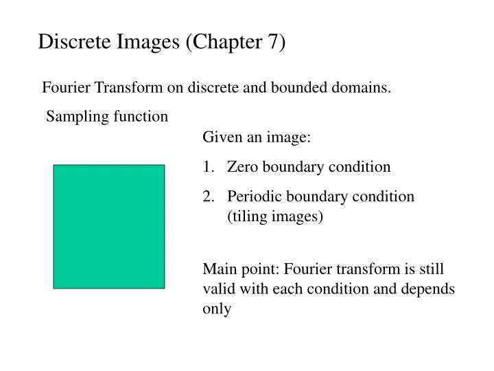
Discrete Images (Chapter 7). Fourier Transform on discrete and bounded domains. Sampling function. Given an image: Zero boundary condition Periodic boundary condition (tiling images) . Main point: Fourier transform is still valid with each condition and depends only .

E N D
Discrete Images (Chapter 7) Fourier Transform on discrete and bounded domains. Sampling function • Given an image: • Zero boundary condition • Periodic boundary condition (tiling images) Main point: Fourier transform is still valid with each condition and depends only
Mathematics in Chapter 7 can look heavy at times…. But don’t get bogged down by the symbols and notations !! For example, the Fourier transform of a periodic function is discrete.
Sampling Theorem If the Fourier transform of a function is bandlimited, then, it can be reconstructed from samples on a regular grid. If Then f(u, v) can be recovered by knowing the values for all k, l
Conversely If the signal is known to be bandlimited with the wavelengh of the highest frequency present Then the sampling interval should be less than In particular, if is the sampling interval, then the signal can contain frequencies only up to the Nyquist frequency If it is to be faithfully reconstructed from Samples.
Edge and Edge Detection February 6
Edges (or Edge points) are pixels at or around which the image values undergo a sharp variation. Edge Detection: Given an image corrupted by acquisition noise, locate the edges most likely to be generated by scene elements, not by noise.
Edge Formation: • Occluding Contours • Two regions are images of two different surfaces • Discontinuity in surface orientation or reflectance properties
More Realistically, due to blurring and noise, we generally have
Image Gradients The gradient of a differentiable function I gives the direction in which the values of the function change most rapidly. Its magnitude gives you the rate of change.
Approximating Derivatives The discrete Laplacian is given as 1 1 -4 1 1
Local Operators (Differential Operators) accentuate noise !! (why?) Therefore, need smoothing before computing image gradients. Motivation: Smoothing removes local intensity variation and what remains are the prominent edges. Gaussian Smoothing with exponential kernel function
Three Steps of Edge Detection • Noise Smoothing: Suppress as much of the image noise as possible. In the absence of specific information, assume the noise white and Gaussian • Edge Enhancement: Designe a filter responding to edges. The filter’s output is large at edge pixels and low elsewhere. Edges can be located as the local maxima in the filters’ output. • Edge Localization: Decide which local maxima in the filter’s output are edges and which are just caused by noise. • Thinning wide edges to 1-pixel with (nonmaximum suppression); • Establishing the minimum value to declare a local maximum an edge (thresholding)
Edge Descriptors (The output of an edge detector) • Edge normal: The direction of the maximum intensity variation at the edge point. • Edge direction: The direction tangent to the edge. • Edge Position : The location of the edge in image • Edge strength: A measure of local image contrast. How significance the intensity variation is across the edge.
Canny Edge Detector (smoothing and enhancement) CANNY_ENHANCER Given image I • Apply Gaussian Smoothing to I. • For each pixel (i, j): • Compute the gradient components • Estimate the edge strength • Estimate the orientation of the edge normal
Canny Edge Detector (Nonmaximum suppression) The input is the output of CANNY_ENHANCER. We need to thin the edges. Given Es, Eo, the edge strength and orientation images. For each pixel (i, j), • Find the direction best approximate the direction Eo(i, j). • If Es(i, j) is smaller than at least one of its two neighbors along this direction, suppress this pixel. The output is an image of the thinned edge points after suppressing nonmaxima edge points.
Canny Edge Detector (Hysteresis Thresholding) Performs edge tracking and reduces the probability of false contours. Input I is the output of nonmaximum_suppression, Eo and two threshold parameters Scan I in a fixed order: • Locate the next unvisited edge pixel (i, j) such that I(i, j) • Starting from (I, j), follow the chains of connected local maxima in both directions perpendicular to the edge normal as long as I • Marked all visited points and save a list of the locations of all points in the connected contour found.