Download
1 / 36
360 likes | 531 Views
Computer Graphics Global Illumination: Monte-Carlo Ray Tracing and Photon Mapping Lecture 11 Taku Komura. In the last lecture . We did ray tracing and radiosity Ray tracing is good to render specular objects but cannot handle indirect diffuse reflections

E N D
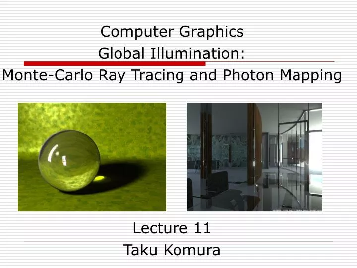
Computer Graphics Global Illumination: Monte-Carlo Ray Tracing and Photon Mapping Lecture 11 Taku Komura
In the last lecture • We did ray tracing and radiosity • Ray tracing is good to render specular objects but cannot handle indirect diffuse reflections • Radiosity can render indirect diffuse reflections but not specular reflections • Both can be combined to synthesize photo-realistic images • But radiosity is very slow and problems with parallelisation • And cannot handle caustics well
Today • Other practical methods to synthesize photo-realistic images • Monte-Carlo Ray Tracing • Path Tracing • Bidirectional Path Tracing • Photon Mapping
Monte-Carlo Ray Tracing :Path Tracing • Start from the eye • When hitting a diffuse surface, pick one ray at random • Otherwise, follow the ordinary ray-tracing procedure • Trace many paths per pixel (100-10000 per pixel) • by Kajiya, SIGGRAPH 86
Shadow ray towards the light at each vertex • Cast an extra shadow ray towards the light source at each step in path • Produce a shadow ray
Path Tracing : algorithm Render image using path tracing for each pixel color = 0 For each sample pick ray in pixel color = color + trace(ray) pixel_color = color/#samples trace(ray) find nearest intersection with scene compute intersection point and normal color = shade (point, normal) return color Shade ( point, normal ) color = 0 for each light source test visibility on light source if visible color=color+direct illumination color = color + trace ( a randomly reflected ray) return color
Path tracing : problems • Vulnerable to noise – need many samples • Using too few paths per pixel result in noise • Difficulty rendering caustics - paths traced only from the camera side • The path needs to go through a number of specular surfaces before hitting the light • Less likely to happen
Examples Jensen, Stanford
Bidirectional Path Tracing • Send paths from light source, record path vertices • Send paths from eye, record path vertices • Connect every vertex of eye path with every vertex in light path • Lafortune & Willems, Compugraphics ’93, Veach & Guibas, EGRW 94
Computing the pixel color • The colour of the pixel can be computed by the weighted sum of contributions from all paths
In what case it works better than path tracing? • Caustics • Indoor scenes where indirect lighting is important • Bidirectional methods take into account the inter-reflections at diffuse surfaces • When the light sources are not easy to reach from the eye
Summary for Monte Carlo Ray tracing • Can simulate caustics • Can simulate bleeding • Requires a lot of samples per pixel
Today : Global Illumination Methods • Monte-Carlo Ray Tracing • Photon Mapping
Photon Mapping • A fast, global illumination algorithm based on Monte-Carlo method • Casting photons from the light source, and • saving the information of reflection in the “photon map”, then • render the results • A stochastic approach that estimates the radiance from limited number of samples http://www.cc.gatech.edu/~phlosoft/photon/
Photon Mapping • A two pass global illumination algorithm • First Pass - Photon Tracing • Second Pass - Rendering
Photon Tracing • The process of emitting discrete photons from the light sources and • tracing them through the scene
Photon Emission • A photon’s life begins at the light source. • Different types of light sources • Brighter lights emit more photons
Photon Scattering • Emitted photons are scattered through a scene and are eventually absorbed or lost • When a photon hits a surface we can decide how much of its energy is absorbed, reflected and refracted based on the surface’s material properties
What to do when the photons hit surfaces • Attenuate the power and reflect the photon • For arbitrary BRDFs • Use Russian Roulette techniques • Decide whether the photon is reflected or not based on the probability
Review : Bidirectional Reflectance Distribution Function (BRDF) • The reflectance of an object can be represented by a function of the incident and reflected angles • This function is called the Bidirectional Reflectance Distribution Function (BRDF) • where E is the incoming irradiance and L is the reflected radiance
Arbitrary BRDF reflection • Can randomly calculate a direction and scale the power by the BRDF
Russian Roulette • If the surface is diffusive+specular, a Monte Carlo technique called Russian Roulette is used to probabilistically decide whether photons are reflected, refracted or absorbed. • Produce a random number between 0 and 1 • Determine whether to transmit, absorb or reflect in a specular or diffusive manner, according to the value
Diffuse and specular reflection • If the photon is to make a diffuse reflection, randomly determine the direction • If the photon is to make a specular reflection, reflect in the mirror direction
Probability of diffuse and specular reflection, and absorption • Probability of reflection can be the maximum energy in any colour band • The probability of diffuse reflection is • Similarly, the probability of specular reflection is
Power adjusted after reflectance • The power Pref of the reflected photon is: Pref,sr = Pinc,r sr / Ps Pref,sg = Pinc,g sg / Ps Pref,sb = Pinc,b sb / Ps where Pinc is the power of the incident photon. The above equation is for specular reflection, but so the same for diffusive reflection
Photon Map • When a photon makes a diffuse bounce, the ray intersection is stored in memory • 3D coordinates on the surface • Colour intensity • Incident direction • The data structure of all the photons is called Photon Map • The photon data is not recorded for specular reflections
Second Pass – Rendering • Finally, a traditional ray tracing procedure is performed by shooting rays from the camera • At the location the ray hits the scene, a sphere is created and enlarged until it includes N photons
Radiance Estimation • The radiance estimate can be written by the following equation
Saving photons:KD tree • The photon maps are classified and saved in a KD-tree • KD-tree : • dividing the samples at the median • The median sample becomes the parent node, and the larger data set form a right child tree, the smaller data set form a left child tree • Further subdivide the children trees • Can efficiently find the neighbours when rendering the scene
Saving photons:Spatial Hashing • Produce a 3D grid • Create a hash function that maps each grid to a list that saves the photons • Scan the photons in the list to find those close to the sample point
NN-search in the grids • Decide the maximum radius of search • Examine the distance between the sample point and the photons in the grid • Gradually increase the radius, search in all the reachable grids until all the photons are found • Suitable for hardware implementation • “Photon Mapping on Programmable Graphics Hardware”, Proceedings of the ACM SIGGRAPH/EUROGRAPHICS Conference on Graphics Hardware, pp. 41-50, 2003
Precision • The precision of the final results depends on • the number of photons emitted • the number of photons counted for calculating the radiance
By 10000 photons and 50 samples(left), and 500000 photons and 500 samples (right)
http://graphics.ucsd.edu/~henrik/animations/jensen-the_light_of_mies_small.mpghttp://graphics.ucsd.edu/~henrik/animations/jensen-the_light_of_mies_small.mpg http://graphics.ucsd.edu/~henrik/animations/jensen-the_light_of_mies_small.avi
Summary • Photon Mapping • A stochastic approach that estimates the radiance from a limited number of photons • Requires less computation comparing to path tracing
Readings • Realistic Image Synthesis Using Photon Mapping by Henrik Wann Jensen, AK Peters • Global Illumination using Photon Maps (EGRW ‘96) Henrik Wann Jensen • Caustics Generation by using Photon Mapping, Presentation by Michael Kaiser and Christian Finger • A Practical Guide to Global Illumination using Photon Maps • Siggraph 2000 Course 8 • http://graphics.stanford.edu/courses/cs348b-01/course8.pdf