Download
1 / 33
330 likes | 401 Views
Learn about different shading models for polygons, including Gouraud and Phong shading techniques. Understand the nuances of constant, interpolated, and smooth shading methods in OpenGL. Explore the concepts of lighting calculations per pixel and bilinear interpolation for realistic rendering. Discover the advanced technique of ray tracing for achieving better realism and sophisticated lighting effects.

E N D
SHADING MODELS FOR POLYGONS Lights @ 2017 by Jim X. Chen: jchen@cs.gmu.edu
Vertex Color • Vertex color can be • specified • calculated according to a lighting model • The normal of each vertex cab be • specified • calculated, for example, by averaging the normals of the polygons sharing the vertex @ 2017 by Jim X. Chen: jchen@cs.gmu.edu
Constant Shading in Old OpenGL • also know as flat shading glShadeModel(GL_FLAT), only one color in a primitive (the last vertex in a primitive) • Valid if the light source & the viewer are at infinity, and the polygon is NOT an approximation of a curved surface. @ 2017 by Jim X. Chen: jchen@cs.gmu.edu
Polygon-Mesh Shading • When approximate a curved surface by a polygonal mesh, using a finer mesh turns out to be ineffective • When the light source is not at infinity, or the viewer is local, flat shading is not quite right • Solution: interpolated shading • Gouraud shading (smooth shading) • Phong shading (normal interpolation) @ 2017 by Jim X. Chen: jchen@cs.gmu.edu
Gouraud Shading • Also called smooth shading, intensity interpolation shading or color interpolation shading, glShadeModel(GL_SMOOTH) • each polygon is shaded by linear interpolation of vertex intensities along each edge and then between edges along each scan line. • The interpolation along edges can easily be integrated with the scan-line visible-surface algorithm. @ 2017 by Jim X. Chen: jchen@cs.gmu.edu
Gouraud Shading • Bilinearly Interpolate Colors at Vertices Down and Across Scan Lines I1 α β γ I2 I3 @ 2017 by Jim X. Chen: jchen@cs.gmu.edu
I= [1 + (N.L) + (max(R.V, 0))2]/3 IA = [1 + cos(60degree) + 0]/3 IB = [1 + cos(60degree) + 0]/3 Ic = [1 + 1 + 1]/3 @ 2017 by Jim X. Chen: jchen@cs.gmu.edu
Phong Shading • Also known as normal-vector interpolation shading • interpolates the surface normal vector rather than the color. • interpolation occurs between vertices, and then across a polygon span on a scan line • Pixel color is calculated using the interpolated normal @ 2017 by Jim X. Chen: jchen@cs.gmu.edu
One Lighting Calculation per Pixel • Approximate surface normals for points inside polygons by bilinear interpolation of normals from vertices N1 Viewer Light N V L N2 N3 Polygon @ 2017 by Jim X. Chen: jchen@cs.gmu.edu
Bilinearly Interpolate Normals at Vertices Down and Across Scan Lines N1 α β γ N2 N3 @ 2017 by Jim X. Chen: jchen@cs.gmu.edu
GLSL/OpenGL 4.x • Send vertex normals to the vertex shader • Normals are transformed by the inverse-transpose of the current matrix • Normals are then sent to fragment shaders (after primitive assembly & interpolation) • Light source and material properties are sent to the fragment shader • Final colors are calculated in the corresponding fragment shaders @ 2017 by Jim X. Chen: jchen@cs.gmu.edu
Gouraud shading v.s. Phong shading • Gouraud shading • if a light source does not cover a vertex, the lighting is missing. • if a highlight fails to fall at a vertex, the specular reflection is missing. • Phong shading • allows a light source covers a polygon’s interior. • allows specular reflection to be located in a polygon’s interior. @ 2017 by Jim X. Chen: jchen@cs.gmu.edu
Shading Comparison Wireframe Flat Phong Gouraud @ 2017 by Jim X. Chen: jchen@cs.gmu.edu
RAY TRACING • Ray tracing is anadvanced global lighting and rendering model that achieve better realism • A ray is sent from the view point through a pixel on the projection plane to the scene @ 2017 by Jim X. Chen: jchen@cs.gmu.edu
Ray tracing is calculated in the device coordinates. So you can consider this is after viewport transformation. • The easiest is to avoid any transformation and viewing, so the models are specified in the device coordinates. @ 2017 by Jim X. Chen: jchen@cs.gmu.edu
Feeler ray to light source for blocking (shadow ray) • Reflected ray for reflection from other objects • Transmitted ray for transparency and refraction @ 2017 by Jim X. Chen: jchen@cs.gmu.edu
Lighting is calculated at each point of intersection. • The final pixel color is an accumulation of all fractions of intensity values from the bottom up. • Rays (named feeler rays or shadow rays) are fired from the point under consideration to the light sources: Li = 0 if light source blocked • The reflection and transmission components at the point are calculated by recursive calls K 1 – å I = I + f f I + + I I e atti spoti Li r t l l l l l i 0 = where Ilraccounts for the reflected light component, and Ilt accounts for the transmitted light component @ 2017 by Jim X. Chen: jchen@cs.gmu.edu
The reflected light component • Ilr is a specular component calculated recursively by the above Equation. • Here, the “view point” is the starting point of the reflected ray: I = M I r s l l l where Mlsis the “view point” material’s specular property. @ 2017 by Jim X. Chen: jchen@cs.gmu.edu
The transmitted light component • The transmission component Ilt is calculated similarly: I = M I t t l l l where Mltis the “view point” material’s transmission coefficient. • The recursion terminates when a user defined depth is achieved or when the reflected and transmitted rays don’t hit objects. • Computing the intersections of the ray with the objects and the normals is the major part of a ray tracing program, which may take hidden surface removal, refractive transparency, and shadows into its implementation considerations. @ 2017 by Jim X. Chen: jchen@cs.gmu.edu
Ray/Sphere Intersection • A sphere equation(x-xc)2+ (y-yc)2 + (z-zc)2 = r2 • A 3D line equation x = x0 +(x1- x0); y = y0 + t(y1- y0); z = z0 + t(z1- z0); • The intersection: solve for t • t2 + Bt + C = 0; @ 2017 by Jim X. Chen: jchen@cs.gmu.edu
Basic Ray Tracing Algorithm • For Each Pixel Ray • Primary ray • Test each surface if it is intersected • Intersected: Secondary ray • Reflection ray • Transparent – Refraction ray @ 2017 by Jim X. Chen: jchen@cs.gmu.edu
Basic Ray Tracing Algorithm • For Each Pixel Ray • Primary ray • Test each surface if it is intersected • Intersected: Secondary ray • Reflection ray • Transparent – Refraction ray @ 2017 by Jim X. Chen: jchen@cs.gmu.edu
Ray Tracing Tree • Ray tree represents illumination computation • One branch reflection • The other branch transmission • Terminated reach the preset maximum, no intersection (background), or strike a “light source” @ 2017 by Jim X. Chen: jchen@cs.gmu.edu
Ray Tracing Tree • Ray tree represents illumination computation Scene Ray Tree @ 2017 by Jim X. Chen: jchen@cs.gmu.edu
Pixel intensity • Sum of intensities at root node • Start at terminal node • If no surfaces are intersected, the intensity of background Ray Tree Ipixel Iback Iback Iback @ 2017 by Jim X. Chen: jchen@cs.gmu.edu
J3_11_rayTracing Recursive Raytracing Example 1. access a pixel in the viewport public void reshape(GLAutoDrawable glDrawable, int x, int y, int w, int h) { gl.glMatrixMode(GL.GL_PROJECTION); gl.glLoadIdentity(); gl.glOrtho(-WIDTH / 2, WIDTH / 2, -HEIGHT / 2, HEIGHT / 2, -4 * HEIGHT, 4 * HEIGHT); gl.glViewport(0,0, WIDTH, HEIGHT); gl.glDisable(GL.GL_LIGHTING); // calculate color by ray tracing gl.glMatrixMode(GL.GL_MODELVIEW); gl.glLoadIdentity(); } @ 2017 by Jim X. Chen: jchen@cs.gmu.edu
2. Initialize objects and light sources // initialize 'ns' number of spheres for (int i = 0; i < ns; i++) { sphere[i][0] = 10 + WIDTH * Math.random() / 10; // radius for (int j = 1; j < 4; j++) { // center sphere[i][j] = -WIDTH / 4 + WIDTH * Math.random() / 2; } } // initialize 'nl' light source locations for (int i = 0; i < nl; i++) { for (int j = 0; j < 3; j++) { // light source positions lightSrc[i][j] = -10 * WIDTH + 20 * WIDTH * Math.random(); } } @ 2017 by Jim X. Chen: jchen@cs.gmu.edu
3. Firing the ray public void display(GLAutoDrawable glDrawable) { // starting viewpoint on positive z axis viewpt[0] = 0; viewpt[1] = 0; viewpt[2] = 1.5*HEIGHT; // trace rays against the spheres and a plane for (double y = -HEIGHT / 2; y < HEIGHT / 2; y++) { for (double x = -WIDTH / 2; x < WIDTH / 2; x++) { // ray from viewpoint to a pixel on the screen raypt[0] = x; raypt[1] = y; raypt[2] = 0; // tracing ray (viewpt to raypt) for depth bounces rayTracing(color, viewpt, raypt, depth); gl.glColor3dv(color, 0); drawPoint(x, y); }}} @ 2017 by Jim X. Chen: jchen@cs.gmu.edu
4. Bounces // recursive rayTracing from vpt to rpt for depth bounces, finding final color public void rayTracing(double[] color, double[] vpt, double[] rpt, int depth) { for (int i = 0; i < 3; i++) { color[i] = 0; } // if (depth == 0) black color if (depth != 0) {// calculate color intersect(vpt, rpt, p, n, depth); // intersect at p with normal n // view direction vector for lighting and reflection for (int i = 0; i < 3; i++) { vD[i] = vpt[i] - rpt[i]; } phong(color, p, vD, n); // current point’s color without reflec. & trans. // reflected ray reflect(vD, n, rD); for (int i = 0; i < 3; i++) { rpoint[i] = rD[i] + p[i]; // a point on the reflected ray starting from p tpoint[i] = -vD[i] + p[i] - n[i]*0.2; // transmitted ray } // recursion to find a bounce at lower level rayTracing(reflectClr, p, rpoint, depth - 1); rayTracing(transmitClr, p, tpoint, depth - 1); for (int i = 0; i < 3; i++) { color[i] = color[i] + 0.4*reflectClr[i] + 0.3*transmitClr[i]; } } p rpoint rpt n vpt @ 2017 by Jim X. Chen: jchen@cs.gmu.edu
5. Calculate Intersections public void intersect(double[] vpt, double[] rpt, double[] point, double[] normal) { // calculate and find intersect point and normal // calculate intersection of ray with the closest sphere // Ray equation: // x/y/z = vpt + t*(rpt - vpt); // Sphere equation: // (x-cx)^2 + (y-cy)^2 + (z-cz)^2 = r^2; // We can solve quadratic formula for t and find the intersection // t has to be > 0 to intersect with an object // return point and normal for intersecting a sphere point[0] = vpt[0] + t * (rpt[0] - vpt[0]); point[1] = vpt[1] + t * (rpt[1] - vpt[1]); point[2] = vpt[2] + t * (rpt[2] - vpt[2]); normal[0] = point[0] - sphere[i][1]; // from the sphere center to the current point normal[1] = point[1] - sphere[i][2]; normal[2] = point[2] - sphere[i][3]; } @ 2017 by Jim X. Chen: jchen@cs.gmu.edu
6. Calculate Lighting public void phong(double[] color, double[] point, double[] vD, double[] n) { for (int i = 0; i < nl; i++) { // if intersect objects between light source, point in shadow intersect(point, lightSrc[i], ipoint, inormal); //a condition whether to calculate light for (int j = 0; j < 3; j++) { lgtsd[j] = lightSrc[i][j] - point[j]; // for light source i // light source direction }normalize(lgtsd); for (int j = 0; j < 3; j++) { s[j] = lgtsd[j] + vD[j]; // for specular term }normalize(s); // for light source i double diffuse = dotprod(lgtsd, n); double specular = Math.pow(dotprod(s, n), 128); if (diffuse < 0)diffuse = 0; if (diffuse==0 || specular < 0) specular = 0; color[0] = color[0] + diffuse + specular; // r, g, b components, this is just r } color[0] = color[0]/nl; //average or normalize by the number of light sources lightSrc n vD point @ 2017 by Jim X. Chen: jchen@cs.gmu.edu
J3_12_SrayTracing Distributed Ray Tracing • averaging multiple rays distributed over an interval; samples randomly chosen points and averages the results • also called stochastic ray tracing. @ 2017 by Jim X. Chen: jchen@cs.gmu.edu
Adaptive Ray Tracing • sample a pixel 4 times in a grid, then compare. • If one sample is different from the others, then subdivide that square recursively • All the samples are close to each other or a predefined depth is reached. The result is a (weighted) average of the samples @ 2017 by Jim X. Chen: jchen@cs.gmu.edu