Download
1 / 87
910 likes | 1.1k Views
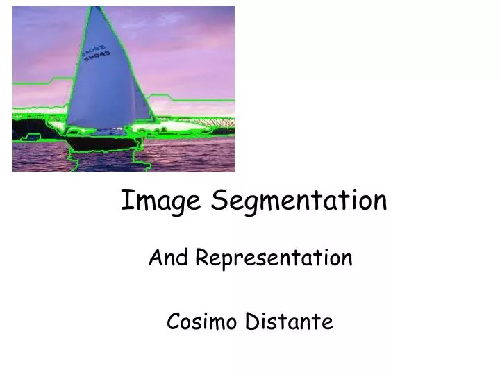
Image Segmentation. And Representation Cosimo Distante. KMeans. Let be the Let us suppose to cluster data inot K classes Let m j , j=1,…,k be the prototype for each class

E N D
Image Segmentation And Representation CosimoDistante
KMeans Let be the Let us suppose to cluster data inot K classes Let mj, j=1,…,k be the prototype for each class Let us suppose having already the K prototypes and we are interested in representing the input data xt with the closest prototype as follow
KMeans How to find the the K prototypes mj? When xt is represented by mi, there is an error proportional to its distance Out objective is to reduce this distance as much as possible Let us introduce an error function (reconstruction)
KMeans Best performances reached by finding the minimum of E Let us use an iterative procedure to find the K prototypes Let’s start by randomly initialize the K prototypes mi Then we compute the b values (membership) and then minimize the errro E by placing the derivative of E to zero Modifying the m values imply that even b values will vary and then the iterative process is repeated until no changes in m will occur
K-Means Clustering • RGB vector
Clustering • Example D. Comaniciu and P. Meer, Robust Analysis of Feature Spaces: Color Image Segmentation, 1997.
K-Means Clustering • Example K=11 K=5 Original
K-means, only color is used in segmentation, four clusters (out of 20) are shown here. EE 7730 - Image Analysis I
K-means, color and position is used in segmentation, four clusters (out of 20) are shown here. Each vector is (R,G,B,x,y). EE 7730 - Image Analysis I
K-Means Clustering: Axis Scaling • Features of different types may have different scales. • For example, pixel coordinates on a 100x100 image vs. RGB color values in the range [0,1]. • Problem: Features with larger scales dominate clustering. • Solution: Scale the features. EE 7730 - Image Analysis I
KMeans Kmeans results with RGB image in. (a) the original image, (b) K=3; (c) K=5;(d)K=6; (e) K=7 and (f) K=8
Fuzzy C-means • Initialize the membership matrix b with values between 0 and 1. such that the following is satisfied • Compute centers mi, i=1,…,k • Compute cost function • Stopping criterion : IF E<threshold or no significative variations between current and previous iteration • Compute the new membership matrix • And goto STEP 2
Contours: Lines and Curves • Edge detectors find “edgels”(pixel level) • To perform imageanalysis : • edges must be grouped into entities such as contours (higher level). • Canny does this to certain extent: the detector finds chains of edgels.
y x Line detection • Mathematical model of a line: Y = mx + n Y1=m x1+n Y2=m x2+n P(x1,y1) P(x2,y2) YN=m xN+n
slope Y = mx + n Y1=m x1+n m’ Y2=m x2+n y n n’ intercept m YN=m xN+n x Parameter Space Image and Parameter Spaces Y = m’x + n’ Image Space Line in Img. Space ~ Point in Param. Space
y x Looking at it backwards … Image space Y = mx + n Fix (m,n), Vary (x,y) - Line Y1=m x1+n Fix (x1,y1), Vary (m,n) – Lines thru a Point P(x1,y1)
m’ n n’ slope m intercept Looking at it backwards … Parameter space Y1=m x1+n Can be re-written as: n = -x1 m + Y1 Fix (-x1,y1), Vary (m,n) - Line n = -x1 m + Y1
Image Space Lines Points Collinear points Parameter Space Points Lines Intersecting lines Img-Param Spaces
Hough Transform Technique • H.T. is a method for detecting straight lines (and curves) in images. • Main idea: • Map a difficult pattern problem into a simple peak detection problem
slope n y n = (-x) m + y intercept m P(x,y) Parameter Space x Hough Transform Technique • Given an edge point, there is an infinite number of lines passing through it (Vary m and n). • These lines can be represented as a line in parameter space.
Hough Transform Technique • Given a set of collinear edge points, each of them have associated a line in parameter space. • These lines intersect at the point (m,n) corresponding to the parameters of the line in the image space.
slope n intercept m Parameter Space n = (-x1) m + y1 y n = (-x2) m + y2 p q P(x1,y1) Q(x2,y2) x
Hough Transform Technique • At each point of the (discrete) parameter space, count how many lines pass through it. • Use an array of counters • Can be thought as a “ parameter image” • The higher the count, the more edges are collinear in the image space. • Find a peak in the counter array • This is a “bright” point in the parameter image • It can be found by thresholding
Practical Issues • The slope of the line is -<m< • The parameter space is INFINITE • The representation y = mx + n does not express lines of the form x = k
y P(x,y) y x x Solution: • Use the “Normal” equation of a line: Y = mx + n = x cos+y sin Is the line orientation Is the distance between the origin and the line
New Parameter Space • Use the parameter space (, ) • The new space is FINITE • 0 < < D , where D is the image diagonal. • 0 < < • The new space can represent all lines • Y = k is represented with = k, =90 • X = k is represented with = k, =0
Consequence: • A Point in Image Space is now represented as a SINUSOID • = x cos+y sin
Hough Transform Algorithm Input is an edge image (E(i,j)=1 for edgels) • Discretize and in increments of d and d. Let A(R,T) be an array of integer accumulators, initialized to 0. • For each pixel E(i,j)=1 and h=1,2,…T do • = i cos(h * d ) + j sin(h * d ) • Find closest integer k corresponding to r • Increment counter A(h,k) by one • Find local maxima in A(R,T)
Hough Transform Speed Up • If we know the orientation of the edge – usually available from the edge detection step • We fix theta in the parameter space and increment only one counter! • We can allow for orientation uncertainty by incrementing a few counters around the “nominal” counter.
Hough Transform for Curves • The H.T. can be generalized to detect any curve that can be expressed in parametric form: • Y = f(x, a1,a2,…ap) • a1, a2, … ap are the parameters • The parameter space is p-dimensional • The accumulating array is LARGE!
Hough Transform for Circles The above equation can be espressed in parametric form
H.T. Summary • H.T. is a “voting” scheme • points vote for a set of parameters describing a line or curve. • The more votes for a particular set • the more evidence that the corresponding curve is present in the image. • Can detect MULTIPLE curves in one shot. • Computational cost increases with the number of parameters describing the curve.
Image matching by Diva Sian by swashford TexPoint fonts used in EMF. Read the TexPoint manual before you delete this box.: AAAAAA
Harder case by Diva Sian by scgbt
Harder still? NASA Mars Rover images
Answer below (look for tiny colored squares…) NASA Mars Rover images with SIFT feature matchesFigure by Noah Snavely