Download
1 / 46
550 likes | 1.05k Views
Capacity Analysis. CE 453 Lecture #14. Objectives. Review LOS definition and determinants Define capacity and relate to “ideal” capacities Review calculating capacity using HCM procedures for basic freeway section Focus on relations between capacity, level-of-service, and design.

E N D
Capacity Analysis CE 453 Lecture #14
Objectives • Review LOS definition and determinants • Define capacity and relate to “ideal” capacities • Review calculating capacity using HCM procedures for basic freeway section • Focus on relations between capacity, level-of-service, and design
Level of Service (LOS) • Concept – a qualitative measure describing operational conditions within a traffic stream and their perception by drivers and/or passengers • Levels represent range of operating conditions defined by measures of effectiveness (MOE)
LOS A (Freeway) • Free flow conditions • Vehicles are unimpeded in their ability to maneuver within the traffic stream • Incidents and breakdowns are easily absorbed
LOS B • Flow reasonably free • Ability to maneuver is slightly restricted • General level of physical and psychological comfort provided to drivers is high • Effects of incidents and breakdowns are easily absorbed
LOS C • Flow at or near FFS • Freedom to maneuver is noticeably restricted • Lane changes more difficult • Minor incidents will be absorbed, but will cause deterioration in service • Queues may form behind significant blockage
LOS D • Speeds begin to decline with increasing flow • Freedom to maneuver is noticeably limited • Drivers experience physical and psychological discomfort • Even minor incidents cause queuing, traffic stream cannot absorb disruptions
LOS E • Capacity • Operations are volatile, virtually no usable gaps • Vehicles are closely spaced • Disruptions such as lane changes can cause a disruption wave that propagates throughout the upstream traffic flow • Cannot dissipate even minor disruptions, incidents will cause breakdown
LOS F • Breakdown or forced flow • Occurs when: • Traffic incidents cause a temporary reduction in capacity • At points of recurring congestion, such as merge or weaving segments • In forecast situations, projected flow (demand) exceeds estimated capacity
Design Level of Service This is the desired quality of traffic conditions from a driver’s perspective (used to determine number of lanes) • Design LOS is higher for higher functional classes • Design LOS is higher for rural areas • LOS is higher for level/rolling than mountainous terrain • Other factors include: adjacent land use type and development intensity, environmental factors, and aesthetic and historic values • Design all elements to same LOS (use HCM to analyze)
Capacity – Defined • Capacity: Maximum hourly rateof vehicles or persons that can reasonably be expected to pass a point, or traverse a uniform section of lane or roadway, during a specified time period under prevailing conditions(traffic and roadway) • Different for different facilities (freeway, multilane, 2-lane rural, signals) • Why would it be different?
Freeways: Capacity (Free-Flow Speed) 2,400 pcphpl (70 mph) 2,350 pcphpl (65 mph) 2,300 pcphpl (60 mph) 2,250 pcphpl (55 mph) Multilane Suburban/Rural 2,200 pcphpl (60 mph) 2,100 (55 mph) 2,000 (50 mph) 1,900 (45 mph) 2-lane rural – 2,800 pcph Signal – 1,900 pcphgpl Ideal Capacity
Principles for Acceptable Degree of Congestion: • Demand <= capacity, even for short time • 75-85% of capacity at signals • Dissipate from queue @ 1500-1800 vph • Afford some choice of speed, related to trip length • Freedom from tension, esp long trips, < 42 veh/mi. • Practical limits - users expect lower LOS in expensive situations (urban, mountainous)
Multilane Highways • Chapter 21 of the Highway Capacity Manual • For rural and suburban multilane highways • Assumptions (Ideal Conditions, all other conditions reduce capacity): • Only passenger cars • No direct access points • A divided highway • FFS > 60 mph • Represents highest level of multilane rural and suburban highways
Multilane Highways • Intended for analysis of uninterrupted-flow highway segments • Signal spacing > 2.0 miles • No on-street parking • No significant bus stops • No significant pedestrian activities
Step 1: Gather data Step 2: Calculate capacity (Supply) Source: HCM, 2000
Lane Width • Base Conditions: 12 foot lanes Source: HCM, 2000
Lane Width (Example) How much does use of 10-foot lanes decrease free flow speed? Flw = 6.6 mph Source: HCM, 2000
Lateral Clearance • Distance to fixed objects • Assumes • >= 6 feet from right edge of travel lanes to obstruction • >= 6 feet from left edge of travel lane to object in median Source: HCM, 2000
Lateral Clearance TLC = LCR + LCL TLC = total lateral clearance in feet LCR = lateral clearance from right edge of travel lane LCL= lateral clearance from left edge of travel lane Source: HCM, 2000
Example: Calculate lateral clearance adjustment for a 4-lane divided highway with milepost markers located 4 feet to the right of the travel lane. TLC = LCR + LCL = 6 + 4 = 10 Flc = 0.4 mph Source: HCM, 2000
fm: Accounts for friction between opposing directions of traffic in adjacent lanes for undivided No adjustment for divided, fm = 1 Source: HCM, 2000
Fa accounts for interruption due to access points along the facility Example: if there are 20 access points per mile, what is the reduction in free flow speed? Fa = 5.0 mph
Estimate Free flow Speed BFFS = free flow under ideal conditions FFS = free flow adjusted for actual conditions From previous examples: FFS = 60 mph – 6.6 mph - 0.4 mph – 0 – 5.0 mph = 48 mph ( reduction of 12 mph)
Step 3: Estimate demand Source: HCM, 2000
Heavy Vehicle Adjustment • Heavy vehicles affect traffic • Slower, larger • fhv increases number of passenger vehicles to account for presence of heavy trucks
f(hv) General Grade Definitions: • Level: combination of alignment (horizontal and vertical) that allows heavy vehicles to maintain same speed as pass. cars (includes short grades 2% or less) • Rolling: combination that causes heavy vehicles to reduce speed substantially below P.C. (but not crawl speed for any length) • Mountainous: Heavy vehicles at crawl speed for significant length or frequent intervals • Use specific grade approach if grade less than 3% is more than ½ mile or grade more than 3% is more than ¼ mile)
Example: for 10% heavy trucks on rolling terrain, what is Fhv? For rolling terrain, ET = 2.5 Fhv = _________1_______ = 0.87 1 + 0.1 (2.5 – 1)
Driver Population Factor (fp) • Non-familiar users affect capacity • fp = 1, familiar users • 1 > fp >=0.85, unfamiliar users
Step 4: Determine LOS Demand Vs. Supply Source: HCM, 2000
Calculate vp • Example: base volume is 2,500 veh/hour • PHF = 0.9, N = 2 • fhv from previous, fhv = 0.87 • Non-familiar users, fp = 0.85 vp = _____2,500 vph _____ = 1878 pc/ph/pl 0.9 x 2 x 0.87 x 0.85
Calculate Density Example: for previous D = _____1878 vph____ = 39.1 pc/mi/lane 48 mph
LOS = E Also, D = 39.1 pc/mi/ln, LOS E
Design Decision • What can we change in a design to provide an acceptable LOS? • Lateral clearance (only 0.4 mph) • Lane width • Number of lanes
Lane Width (Example) How much does use of 10 foot lanes decrease free flow speed? Flw = 6.6 mph Source: HCM, 2000
Recalculate Density Example: for previous (but with wider lanes) D = _____1878 vph____ = 34.1 pc/mi/lane 55 mph
LOS = E Now D = 34.1 pc/mi/ln, on border of LOS E
Recalculate vp, while adding a lane • Example: base volume is 2,500 veh/hour • PHF = 0.9, N = 3 • fhv from previous, fhv = 0.87 • Non-familiar users, fp = 0.85 vp = _____2,500 vph _____ = 1252 pc/ph/pl 0.9 x 3 x 0.87 x 0.85
Calculate Density Example: for previous D = _____1252 vph____ = 26.1 pc/mi/lane 48 mph
LOS = D Now D = 26.1 pc/mi/ln, LOS D (almost C)