Download
1 / 31
310 likes | 324 Views
Sorting (Part I). CSE 373 Data Structures Lecture 13. Reading. Reading Sections 7.1-7.3 and 7.5. Sorting. Input an array A of data records (Note: we have seen how to sort when elements are in linked lists: Mergesort) a key value in each data record

E N D
Sorting (Part I) CSE 373 Data Structures Lecture 13
Reading • Reading • Sections 7.1-7.3 and 7.5 Sorting Part I - Lecture 13
Sorting • Input • an array A of data records(Note: we have seen how to sort when elements are in linked lists: Mergesort) • a key value in each data record • a comparison function which imposes a consistent ordering on the keys(e.g., integers) • Output • reorganize the elements of A such that • For any i and j, if i < j then A[i] A[j] Sorting Part I - Lecture 13
Consistent Ordering • The comparison function must provided a consistent ordering on the set of possible keys • You can compare any two keys and get back an indication of a < b, a > b, or a = b • The comparison functions must be consistent • If compare(a,b) says a<b, then compare(b,a) must say b>a • If compare(a,b) says a=b, then compare(b,a) must say b=a • If compare(a,b) says a=b, then equals(a,b) and equals(b,a) must say a=b Sorting Part I - Lecture 13
Why Sort? • Sorting algorithms are among the most frequently used algorithms in computer science • Allows binary search of an N-element array in O(log N) time • Allows O(1) time access to kth largest element in the array for any k • Allows easy detection of any duplicates Sorting Part I - Lecture 13
Space • How much space does the sorting algorithm require in order to sort the collection of items? • Is copying needed? O(n) additional space • In-place sorting – no copying – O(1) additional space • Somewhere in between for “temporary”, e.g. O(logn) space • External memory sorting – data so large that does not fit in memory Sorting Part I - Lecture 13
Time • How fast is the algorithm? • The definition of a sorted array A says that for any i<j, A[i] < A[j] • This means that you need to at least check on each element at the very minimum, I.e., at least O(N) • And you could end up checking each element against every other element, which is O(N2) • The big question is: How close to O(N) can you get? Sorting Part I - Lecture 13
n2 n·log2n n Faster is better! log2n
Stability • Stability: Does it rearrange the order of input data records which have the same key value (duplicates)? • E.g. Phone book sorted by name. Now sort by county – is the list still sorted by name within each county? • Extremely important property for databases • A stable sorting algorithm is one which does not rearrange the order of duplicate keys Sorting Part I - Lecture 13
Example 5a 8 3a 5b 4 3b 2 3c 5a 8 3a 5b 4 3b 2 3c 2 3a 3b 3c 4 5a 5b 8 2 3c 3b 3a 4 5a 5b 8 Unstable Sort Stable Sort Sorting Part I - Lecture 13
Bubble Sort • “Bubble” elements to to their proper place in the array by comparing elements i and i+1, and swapping if A[i] > A[i+1] • Bubble every element towards its correct position • last position has the largest element • then bubble every element except the last one towards its correct position • then repeat until done or until the end of the quarter, whichever comes first ... Sorting Part I - Lecture 13
Bubblesort bubble(A[1..n]: integer array, n : integer): { i, j : integer; for i = 1 to n-1 do for j = 2 to n–i+1 do if A[j-1] > A[j] then SWAP(A[j-1],A[j]); } SWAP(a,b) : { t :integer; t:=a; a:=b; b:=t; } Sorting Part I - Lecture 13
Put the largest element in its place larger value? 2 3 8 8 1 2 3 8 7 9 10 12 23 18 15 16 17 14 swap 1 2 3 7 8 9 10 12 23 18 15 16 17 14 9 10 12 23 23 1 2 3 7 8 9 10 12 23 18 15 16 17 14 swap 1 2 3 7 8 9 10 12 18 23 15 16 17 14 swap 1 2 3 7 8 9 10 12 18 15 23 16 17 14 swap 1 2 3 7 8 9 10 12 18 15 16 23 17 14 swap 1 2 3 7 8 9 10 12 18 15 16 17 23 14 swap 1 2 3 7 8 9 10 12 18 15 16 17 14 23 Sorting Part I - Lecture 13
Put 2nd largest element in its place larger value? 9 10 12 18 18 2 3 7 8 1 2 3 7 8 9 10 12 18 15 16 17 14 23 swap 1 2 3 7 8 9 10 12 15 18 16 17 14 23 swap 1 2 3 7 8 9 10 12 15 16 18 17 14 23 swap 1 2 3 7 8 9 10 12 15 16 17 18 14 23 swap 1 2 3 7 8 9 10 12 15 16 17 14 18 23 Two elements done, only n-2 more to go ... Sorting Part I - Lecture 13
Bubble Sort: Just Say No • “Bubble” elements to to their proper place in the array by comparing elements i and i+1, and swapping if A[i] > A[i+1] • We bubblize for i=1 to n (i.e, n times) • Each bubblization is a loop that makes n-i comparisons • This is O(n2) Sorting Part I - Lecture 13
Insertion Sort • What if first k elements of array are already sorted? • 4, 7, 12,5, 19, 16 • We can shift the tail of the sorted elements list down and then insert next element into proper position and we get k+1 sorted elements • 4, 5, 7, 12, 19, 16 Sorting Part I - Lecture 13
Insertion Sort InsertionSort(A[1..N]: integer array, N: integer) { i, j, temp: integer ; for i = 2 to N { temp := A[i]; j := i-1; while j > 1 and A[j-1] > temp { A[j] := A[j-1]; j := j–1;} A[j] = temp; } } • Is Insertion sort in place? Stable? Running time = ? • Have we used this before? Sorting Part I - Lecture 13
Example 1 2 3 8 7 9 10 12 23 18 15 16 17 14 1 2 3 7 8 9 10 12 23 18 15 16 17 14 1 2 3 7 8 9 10 12 18 23 15 16 17 14 1 2 3 7 8 9 10 12 18 15 23 16 17 14 1 2 3 7 8 9 10 12 15 18 23 16 17 14 1 2 3 7 8 9 10 12 15 18 16 23 17 14 1 2 3 7 8 9 10 12 15 16 18 23 17 14 Sorting Part I - Lecture 13
Example 1 2 3 7 8 9 10 12 15 16 18 17 23 14 1 2 3 7 8 9 10 12 15 16 17 18 23 14 1 2 3 7 8 9 10 12 15 16 17 18 14 23 1 2 3 7 8 9 10 12 15 16 17 14 18 23 1 2 3 7 8 9 10 12 15 16 14 17 18 23 1 2 3 7 8 9 10 12 15 14 16 17 18 23 1 2 3 7 8 9 10 12 14 15 16 17 18 23 Sorting Part I - Lecture 13
Insertion Sort Characteristics • In place and Stable • Running time • Worst case is O(N2) • reverse order input • must copy every element every time • Good sorting algorithm for almost sorted data • Each item is close to where it belongs in sorted order. Sorting Part I - Lecture 13
Inversions • Aninversion is a pair of elements in wrong order • i < j but A[i] > A[j] • By definition, a sorted array has no inversions • So you can think of sorting as the process of removing inversions in the order of the elements Sorting Part I - Lecture 13
Inversions • A single value out of place can cause several inversions 1 2 3 8 7 9 10 12 23 14 15 16 17 18 value index 8 9 10 11 12 13 0 1 2 3 4 5 6 7 Sorting Part I - Lecture 13
Reverse order • All values out of place (reverse order) causes numerous inversions 1 2 3 8 7 9 10 12 23 18 17 16 15 14 value index 8 9 10 11 12 13 0 1 2 3 4 5 6 7 Sorting Part I - Lecture 13
Inversions • Our simple sorting algorithms so far swap adjacent elements (explicitly or implicitly) and remove just 1 inversion at a time • Their running time is proportional to number of inversions in array • Given N distinct keys, the maximum possible number of inversions is Sorting Part I - Lecture 13
Inversions and Adjacent Swap Sorts • "Average" list will contain half the max number of inversions = • So the average running time of Insertion sort is (N2) (i.e, O(N2) is a tight bound) • Any sorting algorithm that only swaps adjacent elements requires (N2) time because each swap removes only one inversion (lower bound) Sorting Part I - Lecture 13
Heap Sort • We use a Max-Heap • Root node = A[1] • Children of A[i] = A[2i], A[2i+1] • Keep track of current size N (number of nodes) 7 7 5 6 2 4 5 6 value index 1 2 3 4 5 6 7 8 2 4 N = 5 Sorting Part I - Lecture 13
Using Binary Heaps for Sorting • Build a max-heap • Do N DeleteMax operations and store each Max element as it comes out of the heap • Data comes out in largest to smallest order • Where can we put the elements as they are removed from the heap? 7 Build Max-heap 5 6 2 4 DeleteMax 6 5 4 2 7 Sorting Part I - Lecture 13
1 Removal = 1 Addition • Every time we do a DeleteMax, the heap gets smaller by one node, and we have one more node to store • Store the data at the end of the heap array • Not "in the heap" but it is in the heap array 6 6 5 4 2 7 value 5 4 index 1 2 3 4 5 6 7 8 2 7 N = 4 Sorting Part I - Lecture 13
Repeated DeleteMax 5 5 2 4 6 7 2 4 1 2 3 4 5 6 7 8 6 7 N = 3 4 4 2 5 6 7 2 5 1 2 3 4 5 6 7 8 6 7 N = 2 Sorting Part I - Lecture 13
Heap Sort is In-place • After all the DeleteMaxs, the heap is gone but the array is full and is in sorted order 2 2 4 5 6 7 value 4 5 index 1 2 3 4 5 6 7 8 6 7 N = 0 Sorting Part I - Lecture 13
Heapsort: Analysis • Running time • time to build max-heap is O(N) • time for N DeleteMax operations is N O(log N) • total time is O(N log N) • Can also show that running time is (N log N) for some inputs, • so worst case is(N log N) • Average case running time is also O(N log N) • Heapsort is in-place but not stable (why?) Sorting Part I - Lecture 13