Download

1 / 49
550 likes | 1.37k Views
Chapter 2 Response to Harmonic Excitation. Introduces the important concept of resonance. 2.1 Harmonic Excitation of Undamped Systems. Consider the usual spring mass damper system with applied force F ( t )= F 0 cos w t w is the driving frequency F 0 is the magnitude of the applied force

E N D
Chapter 2 Response to Harmonic Excitation Introduces the important concept of resonance Mechanical Engineering at Virginia Tech
2.1 Harmonic Excitation of Undamped Systems • Consider the usual spring mass damper system with applied force F(t)=F0coswt • w is the driving frequency • F0 is the magnitude of the applied force • We take c = 0 to start with Displacement x F=F0cost k M Mechanical Engineering at Virginia Tech
Equations of motion Figure 2.1 • Solution is the sum of homogenous and particular solution • The particular solution assumes form of forcing function (physically the input wins): Mechanical Engineering at Virginia Tech
Substitute particular solution into the equation of motion: Thus the particular solution has the form: Mechanical Engineering at Virginia Tech
Add particular and homogeneous solutions to get general solution: Mechanical Engineering at Virginia Tech
Apply the initial conditions to evaluate the constants (2.11) Mechanical Engineering at Virginia Tech
Comparison of free and forced response • Sum of two harmonic terms of different frequency • Free response has amplitude and phase effected by forcing function • Our solution is not defined for wn = w because it produces division by 0. • If forcing frequency is close to natural frequency the amplitude of particular solution is very large Mechanical Engineering at Virginia Tech
Response for m=100 kg, k=1000 N/m, F=100 N, w = wn +5 v0=0.1m/s and x0= -0.02 m. 0.05 0 Displacement (x) -0.05 0 2 4 6 8 10 Time (sec) Note the obvious presence of two harmonic signals Go to code demo Mechanical Engineering at Virginia Tech
What happens when w is near wn? When the drive frequency and natural frequency are close a beating phenomena occurs 1 0.5 0 Displacement (x) Larger amplitude -0.5 -1 0 5 10 15 20 25 30 Time (sec) Mechanical Engineering at Virginia Tech
5 Displacement (x) 0 -5 0 5 10 15 20 25 30 Time (sec) What happens when w is wn? When the drive frequency and natural frequency are the same the amplitude of the vibration grows without bounds. This is known as a resonance condition. The most important concept in Chapter 2! Mechanical Engineering at Virginia Tech
Example 2.1.1:Compute and plot the response for m=10 kg, k=1000 N/m, x0=0,v0=0.2 m/s, F=23 N, w=2wn. Mechanical Engineering at Virginia Tech
Example 2.1.2 Given zero initial conditions a harmonic input of 10 Hz with 20 N magnitude and k= 2000 N/m, and measured response amplitude of 0.1m, compute the mass of the system. Mechanical Engineering at Virginia Tech
Example 2.1.3 Design a rectangular mount for a security camera. Compute l so that the mount keeps the camera from vibrating more then 0.01 m of maximum amplitude under a wind load of 15 N at 10 Hz. The mass of the camera is 3 kg. Mechanical Engineering at Virginia Tech
Solution:Modeling the mount and camera as a beam with a tip mass, and the wind as harmonic, the equation of motion becomes: From strength of materials: Thus the frequency expression is: Here we are interested computing l that will make the amplitude less then 0.01m: Mechanical Engineering at Virginia Tech
Case (a) (assume aluminum for the material): Case (b): Mechanical Engineering at Virginia Tech
Remembering the constraint that the length must be at least 0.5 m, (a) and (b) yield Less material is usually desired, so chose case a, say l = 0.55 m. To check, note that Thus the case a condition is met. Next check the mass of the designed beam to insure it does not change the frequency. Note it is much less then m. Mechanical Engineering at Virginia Tech
A harmonic force may also be represented by sine or a complex exponential. How does thischange the solution? The particular solution then becomes a sine: Substitution of (2.19) into (2.18) yields: Solving for the homogenous solution and evaluating the constants yields Mechanical Engineering at Virginia Tech
Section 2.2 Harmonic Excitation of Damped Systems Extending resonance and response calculation to damped systems Mechanical Engineering at Virginia Tech
Displacement x k F=F0coswt M c 2.2 Harmonic excitation of damped systems Mechanical Engineering at Virginia Tech
Let xp have the form: Note that we are using the rectangular form, but we could use one of the other forms of the solution. Mechanical Engineering at Virginia Tech
Substitute into the equations of motion Mechanical Engineering at Virginia Tech
Write as a matrix equation: Solving for As and Bs: Mechanical Engineering at Virginia Tech
Substitute the values of As and Bs into xp: Add homogeneous and particular to get total solution: Note: that A and f will not have the same values as in Ch 1, for the free response. Also as t gets large, transient dies out. Mechanical Engineering at Virginia Tech
Things to notice about damped forced response • If z = 0, undamped equations result • Steady state solution prevails for large t • Often we ignore the transient term (how large is z, how long is t?) • Coefficients of transient terms (constants of integration) are effected by the initial conditions AND the forcing function • For underdamped systems at resonance the, amplitude is finite. Mechanical Engineering at Virginia Tech
Example 2.2.1: wn = 10 rad/s, w = 5 rad/s, z = 0.01, F0= 1000 N, m = 100 kg, and the initial conditions x0 = 0.05 m and v0 = 0. Compare A and f for forced and unforced case: Using the equations on slide 6: Differentiating yields: The numbers in ( ) are those obtained by incorrectly using the free response values Mechanical Engineering at Virginia Tech
Proceeding with ignoring the transient • Always check to make sure the transient is not significant • For example, transients are very important in earthquakes • However, in many machine applications transients may be ignored Mechanical Engineering at Virginia Tech
Proceeding with ignoring the transient Magnitude: (2.39) Frequency ratio: Non dimensional Form: (2.40) Phase: Mechanical Engineering at Virginia Tech
40 z =0.01 z =0.1 30 z =0.3 z =0.5 20 z =1 X (dB) 10 0 -10 -20 0 0.5 1 1.5 2 r Magnitude plot • Resonance is close to r = 1 • For z = 0, r =1 defines resonance • As z grows resonance moves r <1, and X decreases • The exact value of r, can be found from differentiating the magnitude Fig 2.7 Mechanical Engineering at Virginia Tech
3.5 z =0.01 3 z =0.1 z =0.3 2.5 z =0.5 z =1 2 Phase (rad) 1.5 1 0.5 0 0 0.5 1 1.5 2 r Phase plot • Resonance occurs at f = p/2 • The phase changes more rapidly when the damping is small • From low to high values of r the phase always changes by 1800 or p radians Fig 2.7 Mechanical Engineering at Virginia Tech
Example 2.2.3 Compute max peak by differentiating: (2.41) (2.42) Mechanical Engineering at Virginia Tech
Effect of Damping on Peak Value 30 • The top plot shows how the peak value becomes very large when the damping level is small • The lower plot shows how the frequency at which the peak value occurs reduces with increased damping • Note that the peak value is only defined for values z<0.707 25 20 15 10 5 0 0 0.2 0.4 0.6 0.8 z 1 0.8 0.6 rpeak 0.4 0.2 0 0 0.2 0.4 0.6 0.8 z Fig 2.9 Mechanical Engineering at Virginia Tech
Section 2.3 Alternative Representations • A variety methods for solving differential equations • So far, we used the method of undetermined coefficients • Now we look at 3 alternatives: a geometric approach a frequency response approach a transform approach • These also give us some insight and additional useful tools. Mechanical Engineering at Virginia Tech
2.3.1 Geometric Approach • Position, velocity and acceleration phase shifted each by p/2 • Therefore write each as a vector • Compute X in terms of F0 via vector addition Im C D C E q A B q B Re A Mechanical Engineering at Virginia Tech
Using vector addition on the diagram: At resonance: Mechanical Engineering at Virginia Tech
2.3.2 Complex response method (2.47) (2.48) Real part of this complex solution corresponds to the physical solution Mechanical Engineering at Virginia Tech
Choose complex exponential as a solution (2.49) (2.50) (2.51) (2.52) Note: These are all complex functions Mechanical Engineering at Virginia Tech
Using complex arithmetic: (2.53) (2.54) (2.55) Has real part = to previous solution Mechanical Engineering at Virginia Tech
Comments: • Label x-axis Re(ejwt) and y-axis Im(ejwt) results in the graphical approach • It is the real part of this complex solution that is physical • The approach is useful in more complicated problems Mechanical Engineering at Virginia Tech
Example 2.3.1: Use the frequency response approach to compute the particular solution of an undamped system The equation of motion is written as Mechanical Engineering at Virginia Tech
2.3.3 Transfer Function Method The Laplace Transform • Changes ODE into algebraic equation • Solve algebraic equation then compute the inverse transform • Rule and table based in many cases • Is used extensively in control analysis to examine the response • Related to the frequency response function Mechanical Engineering at Virginia Tech
The Laplace Transform approach: • See appendix B and section 3.4 for details • Transforms the time variable into an algebraic, complex variable • Transforms differential equations into an algebraic equation • Related to the frequency response method Mechanical Engineering at Virginia Tech
Take the transform of the equation of motion: Now solve algebraic equation in s for X(s) To get the time response this must be “inverse transformed” Mechanical Engineering at Virginia Tech
Transfer Function Method With zero initial conditions: The transfer function (2.59) (2.60) Mechanical Engineering at Virginia Tech
Example 2.3.2 Compute forced response of the suspension system shown using the Laplace transform Summing moments about the shaft: Taking the Laplace transform: Taking the inverse Laplace transform: Mechanical Engineering at Virginia Tech
Notes on Phase for Homogeneous and Particular Solutions • Equation (2.37) gives the full solution for a harmonically driven underdamped SDOF oscillator to beHow do we interpret these phase angles?Why is one added and the other subtracted? Mechanical Engineering at Virginia Tech
Non-Zero initial conditions Mechanical Engineering at Virginia Tech
Zero initial displacement Mechanical Engineering at Virginia Tech
Zero initial velocity Mechanical Engineering at Virginia Tech
Phase on Particular Solution • Simple “atan” gives -π/2 < f < π/2 • Four-quadrant “atan2” gives 0 < f < π F0cos(wt) f Xcos(wt-f) f 2zwnw 2zwnw f wt wn2-w2 wn2-w2 w>wn w<wn Mechanical Engineering at Virginia Tech