The BCM theory of synaptic plasticity. The BCM theory of cortical plasticity

1. The BCM theory of synaptic plasticity. The BCM theory of cortical plasticity BCM stands for Bienestock Cooper and Munro, it dates back to 1982. It was designed in order to account for experiments which demonstrated that the development of orientation selective cells depends on rearing in a patterned environment.

2. (Bienenstock, Cooper, Munro 1982; Intrator, Cooper 1992) BCM Theory Requires • Bidirectional synaptic modification LTP/LTD • Sliding modification threshold • The fixed points depend on the environment, and in a patterned environment only selective fixed points are stable. LTD LTP

3. The integral form of the average: Is equivalent to this differential form: Note, it is essential that θm is a superlinear function of the history of C, that is: with p>0 Note also that in the original BCM formulation (1982) rather then

4. What is the outcome of the BCM theory? Assume a neuron with N inputs (N synapses), and an environment composed of N different input vectors. A N=2 example: What are the stable fixed points of W in this case? x1 x2

5. (Notation: ) Note:Every time a new input is presented, m changes, and so does θm x1 x2 What are the fixed points? What are the stable fixed points?

6. Two examples with N= 5 Note: The stable FP is such that for one pattern yi=wTxi=θm while for the othersy(i≠j)=0. Show movie (note: here c=y)

7. BCM TheoryStability • One dimension • Quadratic form • Instantaneous limit

8. BCM TheorySelectivity • Two dimensions • Two patterns • Quadratic form • Averaged threshold , • Fixed points

9. BCM Theory: Selectivity • Learning Equation • Four possible fixed points , (unselective) , (Selective) , (Selective) , (unselective) • Threshold

10. Consider a selective F.P (w1) where: and So that for a small pertubation from the F.P such that The two inputs result in: So that

11. At y≈0 and at y≈θm we make a linear approximation In order to examine whether a fixed point is stable we examine if the average norm of the perturbation ||Δw|| increases or decreases. Decrease ≡ Stable Increase ≡ Unstable

12. Note: for a small perturbation θm changes such that: For the preferred input x1: (show form here up to end of proof + bonus 50 pt) For the non preferred input x2

13. Note: for a small perturbation θm changes such that: For the preferred input x1: (show from here up to end of proof + bonus 25 pt) For the non preferred input x2 (Note O(Δw2) is very small)

14. Use trick: And Insert previous to show that:

15. Phase plane analysis of BCM in 1D Previous analysis assumed that θm=E[y2] exactly. If we use instead the dynamical equation Will the stability be altered? Look at 1D example

16. Phase plane analysis of BCM in 1D Assume x=1 and therefore y=w. Get the two BCM equations: y 1 0.5 0 ? 0 0.5 1 θm There are two fixed points y=0, θm=0, and y=1, θm=1. The previous analysis shows that the second one is stable, what would be the case here? How can we do this? (supplementary homework problem)

17. Linear stability analysis:

18. Summary • The BCM rule is based on two differential equations, what are they? • When there are two linearly independent inputs, what will be the BCM stable fixed points? What will θ be? • When there are K independent inputs, what are the stable fixed points? What will θ be?

19. Homework 2: due in 10 days • Code a single BCM neuron, apply to case with 2 linearly independent inputs with equal probability • Apply to 2 inputs with different probabilities, what is different? • Apply to 4 linearly indep. Inputs with same prob. • Extra credit 25 pt • 4. a. Analyze the f.p in 1D case, what are the stable f.p as a function of the systems parameters. b. Use simulations to plot dynamics of y(t), θ(t) and their trajectories in the m θ plane for different parameters. Compare stability to analytical results (Key parameters, ητ)

20. retinal activity image Natural Images, Noise, and Learning • present patches • update weights Retina • Patches from retinal activity image LGN • Patches from noise Cortex

21. Resulting receptive fields Corresponding tuning curves

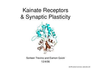
22. 100 50 0 100 50 0 No. of Cells 40 20 0 100 50 0 1 2 3 4 5 Bin Right Eye BCM neurons can develop both orientation selectivity and varying degrees of Ocular Dominance Left Eye Right Synapses Left Synapses Shouval et. al., Neural Computation, 1996

23. Monocular DeprivationHomosynaptic model (BCM) Low noise High noise

24. Monocular DeprivationHeterosynaptic model (K2) Low noise High noise

25. QBCM K1 S1 Noise std Noise std Noise std PCA K2 S2 Noise std Noise std Noise std Noise Dependence of MD Two families of synaptic plasticity rules Homosynaptic Normalized Time Heterosynaptic Normalized Time Blais, Shouval, Cooper. PNAS, 1999

26. I n t r a o c u l a r i n j e c t i o n o f T T X r e d u c e s a c t i v i t y o f t h e " d e p r i v e d - e y e " L G N i n p u t s t o c o r t e x E y e o p e n 3 0 1 5 1 5 c 2 5 e s 1 0 1 0 2 0 / s e 1 5 k i 1 0 5 5 p S 5 0 0 0 0 1 2 0 1 2 0 1 2 LGN R i g h t R e t i n a TTX c l o s e d L i d T i m e ( s e c )

27. Experiment design Blind injection of TTX and lid- suture (P49-61) Dark rearing to allow TTX to wear off Quantitative measurements of ocular dominance

28. Response rate (spikes/sec)

29. Cumulative distribution Of OD MS= Monocular lid suture MI= Monocular inactivation (TTX) Rittenhouse, Shouval, Paradiso, Bear - Nature 1999

30. Why is Binocular Deprivation slower than Monocular Deprivation? Monocular Deprivation Binocular Deprivation

31. What did we learn up to here?